
 Share This Page
| Home | | Mathematics | | * Sage | | | Share This Page |
Profiling the dynamics of a falling body
— P. Lutus — Message Page — Copyright © 2009, P. Lutus(double-click any word to see its definition)
To navigate this multi-page article:Use the drop-down lists and arrow icons located at the top and bottom of each page.

Click here to download the
Sage worksheet used in preparing this article. The Sage worksheet cells in this article should function if pasted into Sage, but if this isn't the case, try downloading the entire worksheet to acquire what may have been inadvertently left out.
This page describes a physics problem that's more difficult than it may seem at first glance, and it presents a challenge for Sage in its present form. Terminal velocity calculations represent a practical use for the Calculus of differential equations, and that's the method we'll be using.
Let me clarify. There are a number of Web resources that provide a terminal velocity number for a given object mass and shape, and there are resources that tell you how long it takes to get to terminal velocity (although some of those results are wrong). But the methods presented here show how to derive an equation that accurately profiles an object's velocity (from zero to terminal) and position with respect to time, then compares the result with published results for the same problem, some correct, some not.
Apart from detailing the calculations behind free-fall, this page is also a Sage tutorial (as are all these pages), so even if the reader has no interest in a skydiver's rapid descent to earth, the methods used to obtain the result may be worth learning.
If we don't take air resistance into account, keeping track of a falling object is trivial — it's a matter of repeated integration. Copy these cell contents into Sage:
# free-fall forms (no air resistance)
var('a,v,p,g,t')
aff(t,g) = -g
vff(t,g) = integrate(aff,t)
pff(t,g) = integrate(vff,t)
show("a(t) = $" + latex(aff(t,g)) + "$")
show("v(t) = $" + latex(vff(t,g)) + "$")
show("p(t) = $" + latex(pff(t,g)) + "$")
(1)
(2)
(3)
We've used Sage to create three functions that can reliably provide acceleration, velocity and position for an object under the influence of gravity, in a place with no air to make things complicated.
In physics, an object's velocity is the time integral of acceleration:(4)And its position is the time integral of velocity: (5)The meaning of the constants k1 and k2 will be explained below.
This is a very simple system — all we need is the value for gravitational acceleration at a particular location and all the other values follow from that. As it turns out, in a vacuum objects of different masses fall at the same rate (because inertial mass and gravitational mass are equal), so in the case of an object falling toward the moon's surface, we have a reliable way to predict its course over time.
Now before we move on the the complexities brought on by air pressure, let's look at the behavior of these functions.
With respect to time, gravitational acceleration is a constant:In a vacuum, velocity increases linearly without bound: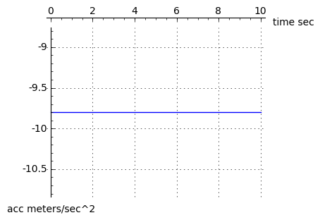 And as shown in equation (3) above, position changes proportional to the square of time:
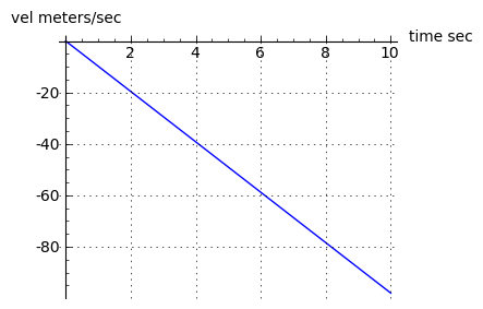
All very simple. But remember for a later discussion, when we introduce air pressure, everything changes.
At this point we need to introduce differential equation (DE) notation:y(t) describes a function whose argument is t. Let's say y(t) represents a vertical position in space and t represents time.
y'(t) (note the apostrophe) represents the first derivative of the function y(t). If y(t) defines a position, then y'(t) defines a velocity.
y''(t) (note the double apostrophe) represents the second derivative of y(t). If y(t) defines a position, then y''(t) defines an acceleration.
It's important to say there are many different notations to describe the relationship between a function and its derivatives. The above is the convention we'll be using in this article, but it is by no means the only way to describe a DE. Also, when we enter a DE into Sage, we have to translate this simple notation into one that is a bit more difficult to use and remember.
A differential equation is expressed as the relationship between a function and one or more of its derivatives. Here's how we would describe the previous section's time/motion equations using DE notation:
Equation number Equation Meaning (4) y''(t) = -g For any time t, the second derivative of position (acceleration) is equal to gravitational constant -g. (5) y'(0) = 0 At time zero, the first derivative of position (velocity) is zero (imagine a skydiver standing in the doorway of an airplane, neither ascending nor descending). (6) y(0) = h At time zero, the position is equal h, or height (the height at which the airplane is flying). Now let's solve this DE using Sage. Remember, Sage's notation is very different from the above:
var('t,g')
y = function('y',t)
de = diff(y,t,2) == -g
soln = desolve(de,[y,t])
show("$y(t) = " + latex(soln) + "$")
(7)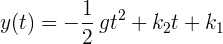
Okay, this result should look familiar from the prior discussion, with a few extra terms. Our differential equation "de" contains one statement — that the second derivative of position is equal to a gravitational constant (equation (4) above), but expressed in the notation Sage requires:
(8) diff(y,t,2) == -g The result provided by "desolve" is correct — it is the result we arrived at earlier using integration (equation (3)) but with two constant terms k1 and k2 included in the result. These terms represent constants of integration: when a function is subjected to indefinite integration, a constant term is assumed to exist, which represents that function's prior history or initial value (equivalent terms). Since our result required two integrations (from acceleration to velocity, then velocity to position), there are two constants of integration. If we choose, we can use k1 and k2 to set initial values for position and velocity respectively. Here is an example:
var('t,g,v_0')
p(t,g,v_0) = soln.subs(k2 == v_0).subs(k1 == 0)
show("$y(t) = " + latex(p(t,g,v_0)) + "$")
plot(p(t,9.8,32),t,0,7,figsize=(4,3),axes_labels=(['Time seconds','Height meters']),gridlines=True)
(9)
In this example, I create a position function p(t,g,v0) that accepts a time argument t, a gravitational acceleration argument g, and an initial velocity argument v0. We can use the initial velocity argument to model the path of a thrown object — let's say at time zero we throw a ball into the air with a vertical velocity component of 32 meters/second — using these assumptions we can submit different time arguments to our function to see when and where the ball lands.
Just for fun, let's see exactly how long the ball stayed aloft — at what time did the ball cross over the zero line on the way down? Here's one way to find out:
find_root(p(t,9.8,32.0),1,8)6.5306122448979593Now for a result that's a bit more subtle — how high did the ball go? Obviously we could apply ½ the result above to our function as a time argument, but remember, we're preparing for problems later on in which there is air resistance and other complicating factors, so let's ignore the true simplicity of this function and pretend it's less well-behaved than it is. Here is one method (not the only one):
top_time = find_root(diff(p(t,9.8,32.0),t),1,8) show(p(top_time,9.8,32.0))52.2448979591837Well, that was a bit tricky. How does it work? Well, the expression "(diff(p(t,9.8,32.0),t)" takes the first derivative of our position function with respect to time, and the first derivative of position is velocity. And as it happens, at the top of the ball's flight, its velocity becomes zero, which allows me to use "find_root" to locate that point. Here is a plot of the ball's velocity on the same scale as the earlier position plot:
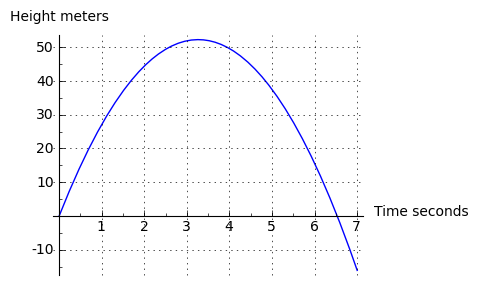
show(diff(p(t,9.8,32),t))
plot(diff(p(t,9.8,32),t),t,0,7,figsize=(4,3),
axes_labels=(['Time seconds','Height meters']),gridlines=True)
(10)
This result shows that the first derivative of our function (the velocity) represents a linear change from +32 (the initial value), through zero, and into negative velocities (meaning the ball is falling back toward the ground). But finding a numerical root is not the simplest or necessarily the best way to locate the top of the ball's flight. Some might even describe it as crude. Here's another way:
solve(diff(p(t,9.8,32),t) == 0,t)[t == (160/49)]Expressed in words, this says, "for the statement p'(t,9.8,32) = 0, what does t equal?" And notice my use of the conventional derivative notation "p'()" to signify the first derivative (which I would love to use in Sage but cannot). Sage's "solve" function has provided a [list] with one element, which we can convert into a floating point number like this:
N(solve(diff(p(t,9.8,32) == 0,t),t)[0].rhs())3.26530612244898This isn't how computer mathematics should be, but it's certainly how it is right now. This entry says, "take the first item in the list ([0]), take the right-hand-side (.rhs()), and turn it into a floating-point number (N(...)).
All right. That should set the stage for the heavy lifting ahead — problems involving air resistance, problems that look more like messy reality.
First, an important physical principle — air resistance increases as the square of velocity. If this were not the case, problems like this would be easy to solve. What this means in practice is that an object falling in air must be modeled using what is technically known as a "second-order nonlinear differential equation." Here are its terms:
Equation number Equation Meaning (11) y''(t) = -g + y'(t)2 k For any time t, the second derivative of position (acceleration) is equal to a gravitational constant -g plus a term that opposes gravitation and is proportional to the square of velocity (y'(t)2) times an empirical factor k that takes the object's cross-sectional area and surface roughness into account. (12) y'(0) = 0 At time zero, the first derivative of position (velocity) is zero (imagine a skydiver standing in the doorway of an airplane, neither ascending nor descending). (13) y(0) = h At time zero, the position is equal h, or height (the height at which the airplane is flying). This is a difficult DE to solve — the second derivative expression not only has the first derivative as one of its terms, but that term is squared and multiplied by a constant k. As it turns out, at the time of writing Sage (version 4.1.2) cannot solve this DE. During the preparation of this article I realized that Sage's DE solver isn't up to processing this complex DE, but because 95% of this article's content can be handled by Sage, I decided to proceed.
Now for the difficult part. I have solved this DE in the past — it's part of my Calculus Tutorial on this site — but for this article I will have my readers click this expression: {y''(t) = -g + y'(t)^2 k,y'(0) = 0,y(0) = h} to get Wolfram Alpha to provide a solution (it's identical to my earlier solution).
I won't pretend not to be amazed by what Wolfram Alpha can do. It's my hope that over time a synergistic process will take place — open-source programs like Sage will match some of Wolfram Alpha's more advanced abilities, and Wolfram Research (creators of Mathematica and Wolfram Alpha) will begin to feel pressure from the world of open source to reduce its prices.Wolfram Alpha provides this solution, as does my earlier work on this problem:
(14)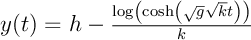
Equation (14) is the position form of the equation — here is the velocity form, the first derivative:
(15)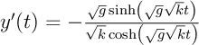
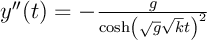
And here is the acceleration form, the second derivative:
(16)
Testing and Comparison
Now I happen to know this solution is correct, but why should you, the reader, accept this on faith? Aren't science and mathematics meant to be endeavors powered by evidence, not faith? So I will try to prove to you that this equation correctly predicts the fall of a body in an atmosphere and represents an exact solution to the differential equation terms laid out above.
We can start by comparing this solution to other published solutions. As it turns out, there are similar forms of this equation — Wikipedia has a nearly identical version in their freefall article — but in an extensive Web search, I have found solutions that aren't obvious equivalents, including some that are simply wrong. Here is one of the wrong equations — we'll be comparing the present equations with this one during a testing phase below:
Source: http://ugrad.math.ubc.ca ... Chapter 11 Notes Equation (located under "11.3 Terminal Velocity"):
(17)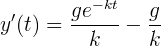
This is a slightly rewritten version of the original — I removed a variable that provided an initial value for velocity, but this change doesn't affect the case of zero initial velocity. Now let's compare the two equations and see if they produce the same results:
var('k')
vf(t,g,k) = -(sqrt(g) * tanh(sqrt(g) * sqrt(k) * t))/sqrt(k)
vubc(t,g,k) = - g/k + (g/k)*e^-(k*t)
g = 9.802 # little-g
tv = -53 # terminal velocity
# acquire k values
ubck = find_root(vubc(100,g,k)==tv,0.001,.2)
vk = find_root(vf(100,g,k)==tv,0.001,.2)
# plot results
pf = plot(vf(t,g,vk),t,0,30)
pubc = plot(vubc(t,g,ubck),t,0,30,rgbcolor='#800000')
# show results
show(pf+pubc,figsize=(4,3),gridlines=True)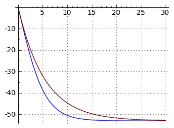
Some explanation is in order:
- Two equations are compared here — equation (15), blue trace, and equation (17) (University of British Columbia), red trace.
- Both equations are meant to provide free-fall velocities as a function of time.
- In order to compare the equations, I needed to choose a single terminal velocity that both equations are expected to arrive at after some time. I chose a descent velocity of 53 meters/second, equal to 118.557 miles per hour, a reasonable approximation of a skydiver's velocity in free-fall.
- In order to make the two equations agree to the degree possible, I needed to compute independent k values for each equation that would produce the specified terminal velocity. As it turns out, the equations cannot be solved for k directly, and further, they do not agree on which k value to use for a given terminal velocity, so I used a root finder approach to arrive at two k values corresponding to 53 meters/second after 100 seconds.
- Applying the two k values and keeping all other conditions the same, I plotted the two equations and overlaid the results.
The two results are very different. This article's equation shows a substantially different profile than the UBC equation. One of these equations is simply wrong. How can we establish which one is wrong? We could collect more equations or we could consult an expert, but those are not particularly good approaches — for one, I have been browsing the Web and found only one other equation that addresses dynamic free-fall (but plenty that predict a final value for terminal velocity). And experts — well, my regular readers may know what I think of experts — I agree with Richard Feynman, who said "Science is the organized skepticism in the reliability of expert opinion".
We should think of a way to compare these equations with each other and with reality. Because Wikipedia has an equation nearly identical to this one, I might conclude that they are valid on the basis of popularity, but that sounds a lot like a combination of logical fallacies (e.g. argumentum ad populum, argumentum ad verecundiam and confirmation bias). So we need some other validation approach.
Numerical Modeling
In applied mathematics there is a time-honored method called "numerical modeling" that can be used to test a theoretical result. I can write a numerical model of the system being evaluated and see if the data from my model agrees with one or the other closed-form equation.
The idea is that a closed-form result (an equation that provides an immediate result for any argument) has it all over a numerical solution for more reasons that I can cover in a finite time interval, but comparison with a numerical model is often a way to detect errors in one's results. Here is my numerical model for the differential equation terms above (11,12,13):
# preliminaries
var('k,t,g')
vf(t,g,k) = -(sqrt(g) * tanh(sqrt(g) * sqrt(k) * t))/sqrt(k)
vubc(t,g,k) = - g/k + (g/k)*e^-(k*t)
g = 9.802 # little-g
tv = -53 # terminal velocity
ubck = find_root(vubc(100,g,k)==tv,0.001,.2)
vk = find_root(vf(100,g,k)==tv,0.001,.2)

# begin numerical model
aarray = []
varray = []
parray = []
# time multiple (increases resolution)
# reduce this number if the algorithm
# takes too long to run
tm = 1000
dt = 1.0/tm # delta time
tt = 30 # total time seconds
na = 0 # acceleration integral
nv = 0 # velocity integral
np = 0 # position integral

for n in range((tt+1)*tm):
    # only print results for integral seconds
    if(n % tm == 0):
        aarray += [na]
        varray += [nv]
        parray += [np]
        # print "t:%2d %12.5f %12.5f %12.5f" % (tt,na,nv,np)
    tt = n*dt
    na = (-g + nv^2 * vk)
    nv += na * dt
    np += nv * dt

# compare numerical result to our equation and UBC equation
lp = list_plot(varray,plotjoined=True,rgbcolor='yellow',linestyle='--')
pf = plot(vf(t,g,vk),t,0,30,rgbcolor='#008000')
pubc = plot(vubc(t,g,ubck),t,0,30,rgbcolor='#800000')
show(pf+pubc+lp,axes_labels=(['Time seconds','Velocity meters']),gridlines=True)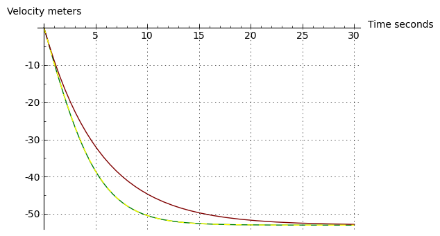
The green-yellow dashed line is the trace shared by equation (15) and the above numerical model's table of results (I show the numerical result as a dashed line so our equation's trace can be seen, otherwise one trace covers the other). This graph shows that the numerical model agrees very well with equation (15). Here is a printed comparison of equation (15) with the numerically derived result, using the data tables generated above:
# print error percent
g = 9.802 # little-g
for tt in range(31):
    ya = varray[tt]
    yb = vf(tt,g,vk)
    ye = 0
    if(tt > 0):
        ye = 100*(ya-yb)/ya
    print "t:%2d %12.5f %12.5f   Error:%8.5f%%" % (tt,ya,yb,ye)
t: 0 0.00000 0.00000 Error: 0.00000% t: 1 -9.69191 -9.69175 Error: 0.00166% t: 2 -18.75689 -18.75631 Error: 0.00306% t: 3 -26.72005 -26.71897 Error: 0.00401% t: 4 -33.33893 -33.33744 Error: 0.00447% t: 5 -38.59217 -38.59043 Error: 0.00451% t: 6 -42.61074 -42.60894 Error: 0.00423% t: 7 -45.59907 -45.59736 Error: 0.00376% t: 8 -47.77484 -47.77330 Error: 0.00322% t: 9 -49.33475 -49.33343 Error: 0.00267% t:10 -50.44080 -50.43971 Error: 0.00216% t:11 -51.21889 -51.21801 Error: 0.00172% t:12 -51.76324 -51.76255 Error: 0.00134% t:13 -52.14260 -52.14206 Error: 0.00104% t:14 -52.40625 -52.40583 Error: 0.00079% t:15 -52.58915 -52.58883 Error: 0.00060% t:16 -52.71586 -52.71562 Error: 0.00045% t:17 -52.80356 -52.80338 Error: 0.00034% t:18 -52.86423 -52.86410 Error: 0.00025% t:19 -52.90618 -52.90608 Error: 0.00019% t:20 -52.93517 -52.93510 Error: 0.00014% t:21 -52.95521 -52.95516 Error: 0.00010% t:22 -52.96906 -52.96902 Error: 0.00007% t:23 -52.97862 -52.97860 Error: 0.00005% t:24 -52.98523 -52.98521 Error: 0.00004% t:25 -52.98980 -52.98978 Error: 0.00003% t:26 -52.99295 -52.99294 Error: 0.00002% t:27 -52.99513 -52.99512 Error: 0.00001% t:28 -52.99664 -52.99663 Error: 0.00001% t:29 -52.99768 -52.99767 Error: 0.00001% t:30 -52.99840 -52.99839 Error: 0.00001%The error terms decline as the number of iterations increases, but the computation time required becomes unacceptable. Typically in numerical modeling, every decimal digit improvement in accuracy requires ten times more processing time. In any case, it seems equation (15) passes this common-sense test — and the UBC equation fails.
As it turns out and after some correspondence, the UBC equation appears to be solving for a case of the Navier-Stokes equations, but this physical model isn't appropriate for a skydiver or other large body falling through a compressible medium like air. Indeed, were it not for the fact that it appears in a section entitled "The skydiver equation," I wouldn't have considered it for an example.
Interestingly, the k value that equation (15) requires to produce a 53 meter/second terminal velocity is also the value required by the numerical model. This suggests the same thing that the numerical comparison does — equation (15) is correct.
Problems in Numerical Models
This numerical modeling business seems terribly inefficient, and it often is, but there are many problems in physics that have no closed-form solutions and that require this sort of brute-force modeling. Examples include:
- The present problem, if gravitational field changes or air pressure changes are allowed to be factors as the problem unfolds. Obviously in a sufficiently large free-fall, both gravitation and air pressure will change.
- Any orbital system with more than two bodies (see the Three-body problem).
- The integral of e-x2, a function that lies at the heart of statistics. Click here: Wolfram Alpha: integrate e^-x^2. This is a well-known example of a function with wide application that cannot be expressed in closed form. When this quantity is required, a numerical estimate is provided by the error function (erf(x)).
- Weather prediction and general environmental modeling. These systems require numerical methods because they are extremely complex and are not representable in closed form. Before the era of supercomputers, such models were of limited value.
An example of the kinds of problems inherent in numerical modeling can be seen in the model above. Examine these two lines from the model:
na = (-g + nv^2 * vk)
nv += na * dt
In this bit of code, na represents the current acceleration value and nv represents the current velocity value. But to compute nv we need the current na value, but to compute na, we need the current nv value — it's a circular reference. Problems like this are common in numerical models, and in this case the obvious solution is to increase the number of iterations to try to minimize the error (by default the above model performs 1000 iterations per modeled second).
More Free-fall Results
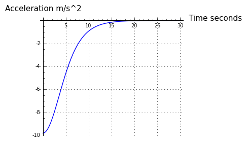
Below are three graphs of the free-fall equation's different forms. First, it makes sense that the acceleration term should have an initial value of 9.8 meters/second, then approach zero as time passes and as air resistance begins to balance gravitation. Let's see:
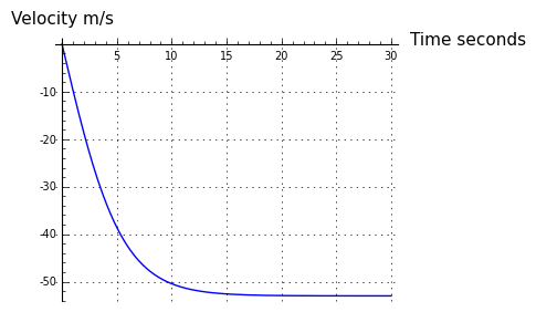
Okay. As to the velocity function, it should start out as a time integral of gravitation (y'(t) = gt) but should become a constant term as air resistance builds up — and it should produce a terminal velocity of 53 meters/second. Let's see:
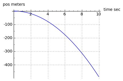
Also okay. The position function should initially change position in a way that reflects the ½ g t2 integral from the no-atmosphere solution, then become a linear descent as the velocity term becomes a constant:
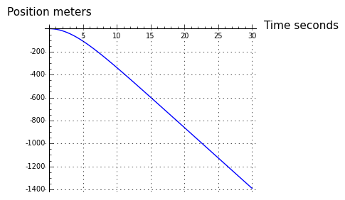
It seems all those graphs closely resemble intuition and reality.
Time to Terminal Velocity
A commonly desired result for this problem is the time required to get to terminal velocity (TV). But this inquiry includes a misconception — the equations we're analyzing never actually get to TV, they only approach it (and this is true in reality as well). Here is a comparison between elapsed time and the proximity of TV, for a TV of 53 meters/second (the elapsed time obviously changes depending on the TV):
var('t,g,k')
vf(t,g,k) = -(sqrt(g) * tanh(sqrt(g) * sqrt(k) * t))/sqrt(k)
g = 9.802
tv = -53
vk = find_root(vf(10000,g,k)==tv,0.001,.2)
for n in range(1,11):
    dv = tv * (1.0-(n/100.0))
    print "Within %2d%% of TV: %6.2f seconds" \
    % (n,find_root(vf(t,g,vk)-dv,1,100))
Within 1% of TV: 14.31 seconds Within 2% of TV: 12.42 seconds Within 3% of TV: 11.31 seconds Within 4% of TV: 10.52 seconds Within 5% of TV: 9.90 seconds Within 6% of TV: 9.40 seconds Within 7% of TV: 8.97 seconds Within 8% of TV: 8.59 seconds Within 9% of TV: 8.26 seconds Within 10% of TV: 7.96 secondsSo the answer to the time-to-TV question is that it depends on what criteria we select, but if we accept a result within 5% of the true value, then ten seconds is a reasonable estimate.
I've always thought a knowledge of differential equations is an essential prerequisite to understanding physics. It is not much of a stretch to say that to a first approximation, modern physics consists of a large set of differential equations.
Sage can solve many kinds of first-order and second-order linear differential equations and has the ability to display its results in a number of useful ways. I find myself using Sage to attack problems that were until now too difficult to express or code. But I look forward to a time when Sage will be able to process a much larger set of equations that lie outside its present comfort zone.
"Exploring Mathematics with Sage" by Paul Lutus is licensed under a
Creative Commons Attribution-Noncommercial-Share Alike 3.0 United States License.
| Home | | Mathematics | | * Sage | | | Share This Page |