

 Share This Page
| Home | | Mathematics | | * Sage | | | | Share This Page |
A matrix-based data analysis method
— P. Lutus — Message Page — Copyright © 2009, P. Lutus(double-click any word to see its definition)
To navigate this multi-page article:Use the drop-down lists and arrow icons located at the top and bottom of each page.
Click here to download the
Sage worksheet used in preparing this article.
This project's Sage code is sufficiently complex that I won't be including an initialization code block on this page as is true for most of the other articles in this set. I highly recommend the above download for those readers who want to explore this topic from a programming perspective. As to the mathematical ideas, I think it should be possible to understand them without benefit of the Sage file.
I'll be including small Sage examples that ought to function without any special initialization, but if this turns out not to be true, I recommend the above download.
The premise of polynomial regression is that a data set of n paired (x,y) members:
(1)
can be processed using a least-squares method to create a predictive polynomial equation of degree p:
(2)
The essence of the method is to reduce the residual R at each data point:
(3)
This is accomplished by first expressing the system in matrix form (this example represents a polynomial of degree 4):
(4)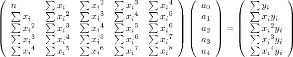
then solving for the unknown middle column, (e.g. a0,a1,a2 ...) by means of Gauss-Jordan elimination. The resulting values represent the polynomial coefficients for equation (2) above.
Programming sidebar: From a programming perspective, each cell in the left-hand square matrix contains this quantity:
(5)
that is to say, the sum of the x values raised to the indicated power, where r equals the matrix row and c the matrix column, each such index in the range 0 <= i <= p, and n equal to the number of data samples. Note also that x0 = 1 and x1 = x.
For those of us who are not direct descendants of Gauss or Euler and who want a deeper understanding of this method, as well as for those who intend to implement this method in computer code, I offer the following detailed procedure with an example data set.
Here is our data:
x y -1 -1 0 3 1 2.5 2 5 3 4 5 2 7 5 9 4 I created this particular data set for its pathological properties and its ability to show what sorts of things can go wrong during efforts to apply polynomial regressions to real-world data.
In my Sage code I create a square matrix equal in size to p+1, p being the solution's desired polynomial degree, then I add an extra column at the right whose purpose will be explained below. For this example, let's choose polynomial degree 4. Referring now to equation (4) above and to the example data set, I perform the operations required to produce this numerical matrix content:
(6)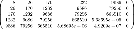
For those who want some insight into the above numbers, here is a Sage cell that generates the matrix data from the x data set provided above:
xvals = [-1,0,1,2,3,5,7,9]
for p in range(9):
    print "%d: %8d" % (p,sum(xvals[n]^p for n in range(len(xvals))))
0: 8 1: 26 2: 170 3: 1232 4: 9686 5: 79256 6: 665510 7: 5686952 8: 49208966In evaluating the matrix shown in equation (4) above, remember that this:
(7)is just a convenient shorthand for this: (8)
(8)
and it means the sum of the squares of the x terms, not the square of the sum.
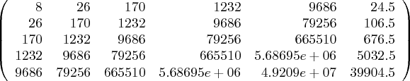
Astute readers will notice I have grafted a column onto the right side of the otherwise self-respecting square matrix in matrix (6) above. This column's purpose is to accommodate the particulars of the Gauss-Jordan elimination (GJE), and we initialize it with the values shown to the right of the equals sign in equation (4) above. At the end of the GJE this column will contain the desired polynomial terms. Here is the matrix with the data added:
(9)
Next we perform a GJE on our matrix. In Sage a Matrix class function called "echelonlize()" can be used to perform this transformation, at the end of which the desired polynomial coefficients will have replaced the right-hand column's original contents, and the original square matrix (the columns to the left of the added column) will be replaced by an identity matrix. Like this:
# reduce matrix
mm=Matrix(RR,m)
mm.echelonize()
(10)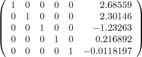
In Sage, we can convert this result into a practical polynomial expression as shown in equation (2) above:
var('x')
y = 0
for j in range(p+1): y += m[j][p]*x^j
show(y)
(11)
The reason for the "var('x')" line above is to assure that x is not defined, as it needs to be an unknown to meet its purpose.
At this stage it would be nice to be able to automate evaluations of our data set and see how the choice of polynomial degree changes the results. The Sage worksheet for this article has a rather nifty interactive graph applet that allows the user to choose different polynomial degrees at will and quickly see a plot of the correlation between the original data and the resulting polynomial equation.
At this stage my readers have a number of choices:
- Run Sage, load the worksheet for this article, and use the graphic applet it contains.
- Open a separate browser tab containing an interactive Java applet on this site named PolySolve that performs the same operations being descibed here.
- Just read along and view the provided graphic images to follow the logic.
Obviously the first choice is to be preferred, but the second choice is a reasonable substitute. Those who click the above PolySolve link using a modern browser will see an new, separate tab open up containing PolySolve, but remember that repeated clicks on the link won't produce the same result as the first one — to view PolySolve after the first click, use the tab, not the link.
The Sage applet in this article's worksheet uses the "@interact" feature to produce an easy-to-change graphic evaluation of our data set. Here is the Sage code and an example graphic:
@interact
def _(p = (0..12)):
    y = polyregress(data,p)
    dp = list_plot([[data[n].x,data[n].y] for n in range(len(data))],rgbcolor='red')
    lp = plot(y,x,list_minmax(data))
    cc = corr_coeff(data,y)
    se = std_error(data,y)
    lbl = text("correlation coefficient (r^2): %f\nStandard error: %f"
    % (cc,se),(5,-2),rgbcolor='black',fontsize=10)
    show(dp+lp+lbl,ymin=-5,ymax=7)
A degree 4 result:
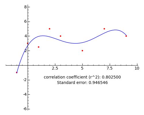
The actual Sage worksheet applet has a slider to choose the polynomial degree, not shown in this graphic.
I want to emphasize that the polynomial regression method described here can be forced to produce perfect agreement with any x,y data set through the simple expedient of choosing a polynomial degree equal to n (the number of data points) - 1. Here is an example (degree 7 for an 8-point data set):
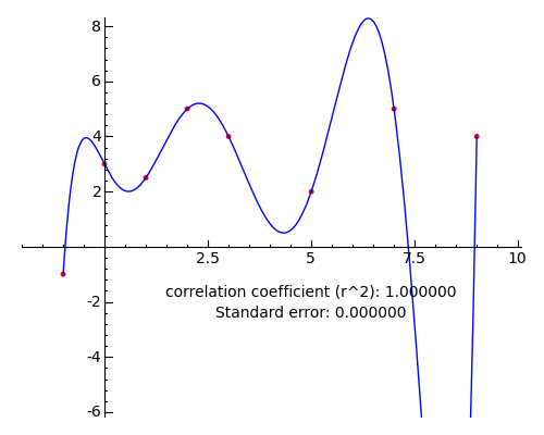
This point cannnot be overemphasized — a polynomial fit can be made perfect by simply increasing the degree of the polynomial, but such a result rarely has meaning. During data evaluations there is a temptation to choose an analysis method that most closely agrees with our preconceived notions about the meaning of the data, but this temptation must be resisted — it represents the dark side of computer-aided data analysis.
People who haven't seen a polynomial data analysis before, and who see a conservative interpretation of a data set like this (degree 1):
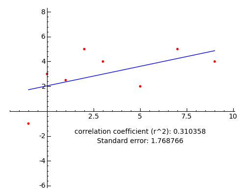
won't necessarily realize that the data may not even support this trend line, much less any higher degree. Notice that the correlation coefficient for this graph is 0.31, rather poor, but the coefficients for all higher degrees are "better", even though they may not represent anything real. Again, one must fight the temptation to create an interpretation that agrees with the analysis, rather than the reverse.
By virtue of the fact that one can select a polynomial degree, polynomial regressions represent a large subset of all regressions, from the simple linear regression form (y = mx + b) to the frequently applied quadratic and cubic regressions. Higher-degree regressions are mostly for entertainment (or mathematical explorations) and have little relevance to the task of producing correlations with data gathered from the real world.
Because it is easy to understand, set up, and solve, this class of regression also serves as an introduction to matrix mathematics, and hopefully will motivate the reader to pursue further activities in this area.
| Home | | Mathematics | | * Sage | | | | Share This Page |