
 Share This Page
| Home | | Python | | | Share This Page |

Installing and using the multi-language Jupyter notebook environment
— P. Lutus — Message Page —
Copyright © 2016, P. Lutus
Most recent update:
(double-click any word to see its definition)
Origin in IPython
Jupyter (http://jupyter.org) is an amazing productivity environment that's under active development and rapidly evolving into a powerful tool for academic and other applications. Jupyter emerged from IPython, an earlier notebook environment that only supported Python activities, but the new scheme, apart from being more advanced, supports many more languages.
Notebooks and Kernels
The basic premise of Jupyter is that a single, well-designed work environment can host any number of language "kernels" or sources of computation and data, for inclusion in content created in the Jupyter notebook interface.
Available Languages
Languages now available include Python (of course), SageMath, Bash, Octave, Julia, Haskell, Ruby, JavaScript, Scala, Erlang, and many more. When installed as Jupyter kernels each language becomes accessible in the same way, using the same notebook interface.
Python/Sympy Example
Jupyter runs a local HTTP server and its notebook environment appears in your browser, where you choose the kernels you want to interact with. Here's an example Python/SymPy notebook session:
NOTE: Each of this page's Jupyter examples can be copied directly from the code cells and pasted into your Jupyter environment for further exploration.
Calculus Example
Here's a more advanced example that solves a second-order differential equation (an example of the so-called "harmonic oscillator" equation):
\begin{equation} y(t) + \frac{d^2}{dt^2}y(t) = 0 \end{equation}Here's the solution and a plot of the result:
Rapid Development
To me personally, Jupyter's real value is shown by the speed with which tasks move forward. I can create notebooks for languages that once required a slow manual cycle of edit, save, execute, repeat. Now I get very fast interactive results in environments that once were notorious time-wasters — like Bash:It's not obvious in the above example, but I can change a few characters and run the code again with a keystroke.
SageMath/Graph Theory
SageMath is a more powerful, but much larger, kernel that can be made available to Jupyter. SageMath is an integrated collection of many mathematical libraries of interest to academics and applied mathematicians, and has a very good symbolic mathematics capability. Here's a SageMath example that shows off an esoteric graphing feature (with an uncommon meaning for the word "graph")*:Notice how each character — including the space — in the test phrase "Natural Selection" appears in the result graph, mapped in a way to avoid multiple appearances of a character used more than once.
Parallel Kernels
It's not apparent from these examples, but one can open multiple notebooks, each running a different Jupyter "kernel," and move between them to take advantage of each one's strengths. In fact, in a project named JupyterLab, this multiple-process idea is being actively pursued. It seems likely that, when fully developed, JupyterLab will replace Jupyter.
For those who find Jupyter intriguing and want a closer look, we can move on to the task of installing Jupyter.
Windows Problems
As is true for many applications and to a greater extent as time passes, installing Jupyter on Linux is much easier than installing it on Windows. The distinction has become so extreme that some kernels/languages (SageMath comes to mind) can only be made accessible in Windows by installing a Linux virtual machine on Windows to host it.
Dessert Before Vegetables (Linux installation)
Let's start with Linux installation, simpler and more flexible than Windows. This example assumes a Ubuntu/Debian environment.
Via Anaconda (installs pretty much everything, for systems with room to grow):
- From this download page, download a package appropriate to your platform (distinguishing between 64 or 32 bit machines and Python versions 3.5 or 2.7).
- Place the downloaded package into any convenient directory.
- Peform an MD5 checksum on the download:
\$ md5sum (package-name)The correct MD5 hashes are
listed here.Proceed with the installation:
System-wide:
As root, create a suitable system-level directory (/opt/anaconda is just an example):
# mkdir /opt/anacondaExecute the Anaconda installer this way:
# bash (Anaconda package name) -p /opt/anacondaAdd the new system-wide binary directory to the system path by editing /etc/environment like this:
PATH=$PATH:/opt/anacondaSingle user:
Create a suitable single-user directory (/home/username/anaconda is just an example, and be sure to replace "username" with your actual user name):
\$ mkdir /home/username/anacondaExecute the Anaconda installer this way:
\$ bash (Anaconda package name) -p /home/username/anacondaAdd the new system-wide binary directory to the system path by editing /home/username/.profile like this:
PATH=$PATH:/home/username/anacondaVia Pip (for fine-tuning and/or for systems with limited storage space):
Install python-pip:
# apt-get install python-pipDecide whether you want a system-wide installation or a single-user installation. For the system-wide installation, precede each of your commands with "
sudo -H". For example, a single-user Jupyter installation would be:\$ pip install jupyterBut a system-wide Jupyter install would be:
\$ sudo -H pip install jupyter
Consult this listand choose which packages to install. Be sure to include the Jupyter package, which will automatically include all its dependencies.For each selected package, install it this way:
Single-user:
\$ pip install (package-name)System-wide:
\$ sudo -H pip install (package-name)For both Anaconda and Pip installations, install desired Jupyter kernels (languages):
Bash
$ sudo -H pip install bash_kernel
$ sudh -H python -m bash_kernel.install
JavaScript
# apt-get install nodejs-legacy npm ipython ipython-notebook libzmq3-dev
# npm install -g ijavascript
$ ijs
Octave
# apt-get install octave
$ sudo -H pip install octave_kernel
$ sudo -H python -m octave_kernel.install
SageMath
This is a very large package, typically greater than 4 GB when unpacked and installed. Sagemath is desirable because it can perform and support more kinds of mathematics than its open-source alternatives, but it's not a small download.
- Install SageMath (this example shows a system-wide installation):
- Choose a download source from this page.
- Copy the source binary's URL for use below.
In a root shell:
# cd /opt
# wget (source URL)
# tar -xjf (downloaded binary name)
The above will create and populate a directory named "SageMath", so the installed system path will be /opt/SageMath.
Add this to /etc/environment:
SAGE_ROOT=/opt/SageMathMake the SageMath kernel visible to Jupyter:
# mkdir -p /usr/local/share/jupyter/kernels
# ln -nsf /opt/SageMath/local/share/jupyter/kernels/sagemath \
/usr/local/share/jupyter/kernels/sagemath
The "mkdir" command is needed because the installed Jupyter won't necessarily have created a "kernels" subdirectory. The symlink command creates a soft link between SageMath and Jupyter, with the advantage that if an update to SageMath changes the contents of the kernel code, this link will still work, but a copy would not benefit from updates.
Again, a SageMath installation will only work on Linux/Solaris/Mac OS X platforms. SageMath isn't available for Windows, but there are strategies to make it available there (below).
- If all the above installation steps are carried out successfully, the install should support a wide range of development activities, and there are more kernels I haven't installed that can expand Jupyter's abilities even further.
Windows Installation
On Windows, a virtual machine is required for access to some Jupyter kernels, but a Python-kernel-only installation is not difficult. All the installations below assume a Windows 10 platform. Let's start with the Python-only install using Anaconda.Via Anaconda (no SageMath support)
Install:
- From this download page, choose a download appropriate to your computer's traits (i.e. 32 or 64 bits) and which Python version you want (most people will want to choose Python 3.5+).
- When the download is complete, run the download and follow the instructions.
- Once the install is complete, a new Anaconda folder will appear in the system applications list, and one of the entries under the Anaconda category will be "Jupyter Notebook". Click and drag this icon from the applications list to your desktop.
- Under the "Documents" folder, create a new folder named "Jupyter". This folder will hold your Jupyter notebooks.
- Returning now to the Jupyter icon you dragged onto your desktop, right-click the icon and choose "Properties."
- In the "Target" entry, use the arrow keys to move to the end of the entry, add a space, and enter this: "c:\users\username\documents\jupyter". Replace "username" with your actual user name. This entry directs Jupyter to put your notebooks in the Jupyter folder you created above. And because the Jupyter data folder is a subfolder of the Documents folder, it will be properly backed up when you back up your personal files. You do back up your personal files, don't you?
Test:
- Click the desktop Jupyter icon.
If the installation has been carried out successfully, the system browser will launch and show something that looks more or less like this:
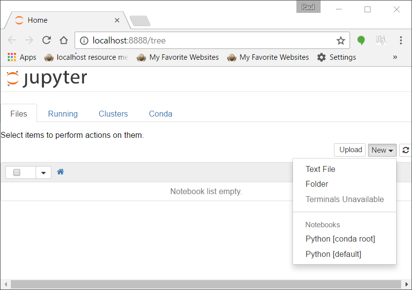
- Click the "New" item at the right (that has its content shown in the above image), and choose one of the Python options — it shouldn't matter which one.
Enter what's shown below (you can copy the contents of the code cell below), then press Ctrl+Enter:
- Your result should resemble that shown above.
- At this stage you should be able to create any of the above examples that involve Python and SymPy.
Via hosted virtual machine (SageMath support)
This installation method requires a SageMath virtual machine installer called the SageAppliance, plus a virtual machine hosting application called VirtualBox.
- Download the SageAppliance from here (which at the time of writing has the name "sage-7.3.ova", always download the most recent version) and put the downloaded archive anywhere convenient.
- Download and install VirtualBox from here — choose a Windows version appropriate to your environment (i.e. 32 or 64 bit).
- Run VirtualBox and select menu item "File ... Import Appliance."
- In the next dialog, navigate to the file downloaded earlier (named "sage-(version).ova") and select it.
- In the next dialog, choose "Import."
- This will import/create a VM named "Sage (version)" the version wil change over time.
Before running the new VM, there are some desirable setting changes:
- Click the entry for the new VM so it's highlighted, then click the toolbar "Settings" icon.
- Choose the System category and increase the amount of system RAM memory made available to the VM if your system will allow it. The default setting of 512 MB is prudent as a default but for a typical modern machine there's more RAM available and Sage will run more efficiently with more RAM. Typically with one running VM, give it half the available RAM.
- Choose the Network category and change the "Attached to" setting to "Bridged Adaptor". This setting will make the virtual machine visible on the host, for reasons explained below.
- Still in the Network category, click "Advanced" and change the "Adaptor Type" to "Paravirtualized Network (virtio-net)". This fixes a Windows 10 compatibility issue.
Now you can start the VM — click the VM entry so it's highlighted, and click the "Start" toolbar button.
- Choose the "New" list at the right of the display, and choose one of the Python options — either one is fine.
- You will see a new, empty Jupyter notebook. Add to it the entries shown below and press Ctrl+Enter.
The next task is to make the Linux VM visible to the Windows host's network (and your local LAN if desired). This isn't likely to be true by default — some additional steps are required:
- First, let's install some important VirtualBox additions into the running VM.
- On the running VM application window, choose menu item "Devices ... Insert Guest Additions CD Image". This will mount a virtual CD containing VirtualBox software that will make the VM more usable.
- Now to gain access to a command line in the Sage guest VM — press the right Ctrl key and function key F1. If this is done correctly, you should see a terminal session with this on display:
sagevm login:- Make the following entries:
sagevm login: root
password: sage
# cd /root
# mkdir mount
# mount /dev/sr0 mount
# cd mount
# ./VboxLinuxAdditions.run
The above will install the VirtualBox guest additions, which greatly increases the chance for a successful network connection between VM and host. NOTE: To exit the command prompt and return to the Jupyter notebook display without having to reboot the VM, press the right Ctrl key and function key F7. Restart the VM to enable the changes. Now (assuming you enabled the "Bridged Adaptor" and "Paravirtualized Network" settings described above) it should be possible to access the virtual machine's Jupyter server from the host Windows machine. Just as a preliminary check in advance of a more elegant solution presented below:
- Run the VM and reacquire the command shell by pressing right-Ctrl plus function key F1 as explained above.
Log in as shown above, then enter this:
# ifconfig- You should see something that looks more or less like this:
# ifconfig
    eth1      Link encap:Ethernet  HWaddr 08:00:27:9B:8D:99
    inet addr:192.168.0.114  Bcast:192.168.0.255  Mask:255.255.255.0
    inet6 addr: fe80::a00:27ff:fe9b:8d99/64 Scope:Link
    UP BROADCAST RUNNING MULTICAST  MTU:1500  Metric:1
    RX packets:4965 errors:0 dropped:0 overruns:0 frame:0
    TX packets:939 errors:0 dropped:0 overruns:0 carrier:0
    collisions:0 txqueuelen:1000
    RX bytes:2357619 (2.2 MiB)  TX bytes:93499 (91.3 KiB)

    lo        Link encap:Local Loopback
    inet addr:127.0.0.1  Mask:255.0.0.0
    inet6 addr: ::1/128 Scope:Host
    UP LOOPBACK RUNNING  MTU:65536  Metric:1
    RX packets:538 errors:0 dropped:0 overruns:0 frame:0
    TX packets:538 errors:0 dropped:0 overruns:0 carrier:0
    collisions:0 txqueuelen:0
    RX bytes:159623 (155.8 KiB)  TX bytes:159623 (155.8 KiB)
Make a note of the four-number address that's highlighted above in red (your numbers probably won't be the same).
- On the host Windows machine, launch a browser and enter this into its address bar:
Replace the example red numbers with the ones you recorded above.http://192.168.0.114:8000The reason for this test is to see if the Jupyter notebook session can be served on the host environment, and in most cases — if all the above settings have been successfully made and there are no unexpected obstacles — the answer will be yes. But a more permanent and flexible solution is available — Zeroconf.
- Zeroconf is a slick network configuration protocol that eliminates complicated setup procedures like the example above. Once Zeroconf has been installed on both Windows and the Linux VM, they can talk to each other very easily, without having to remember any numbers or difficult sequences.
- To make Zeroconf available to Windows, install this package. Because Zeroconf means what it says, there's no setup required — once installed, it will become available.
- It's not normally necessary to install Zeroconf on Linux, because it's usually preinstalled and running, but there are exceptions — like the SageMath Appliance, which was made as small as possible by eliminating all packages not absolutely necessary.
To install Zeroconf on the SageMath virtual machine, acquire a command prompt as shown above, log in, and issue these commands:
# yum install avahi-tools # yum install nss-mdns- Once the above instructions have been issued, Zeroconf is available. From the Windows host, you can now access the Linux Jupyter VM by its new name "sagevm.local", and this will remain true after the numerical address used above has been long forgotten (changed in the normal course of network operations).
- On the host Windows machine, launch a browser and enter this into its address bar:
http://sagevm.local:8000- Apart from being able to choose any host browser for the notebook interface, this network presence means you can upload and download notebooks from the chosen browser, so the problem of importing and exporting files to/from the VM goes away.
- With an appropriate network setup, other machines on your local network can access the Windows-hosted Jupyter VM in the same way.
This completes the installation of Jupyter.
Symbolic mathematics isn't the only purpose served by Jupyter's many available kernels. There are numeric math libraries, statistical libraries/languages and many others, but because symbolic math is an interest of mine, I want to show an example of symbolic equation processing.
In this example we solve a problem of modest difficulty — we take an important multi-variable equation used in financial calculations and use the SymPy symbolic math library to create all its forms.
Future Value Equation
The basic equation from which all the variations emerge is called "Future Value", and it looks like this (for payment at the end of each period): \begin{equation} fv = \frac{1}{ir} \left(- ir \, pv \left(ir + 1\right)^{np} - pmt \left(ir + 1\right)^{np} + pmt\right) \end{equation}Where, with respect to an interest-bearing annuity:
- $fv$ = Future value.
- $pv$ = Present value.
- $pmt$ = Periodic payment/withdrawal.
- $np$ = Number of payments.
- $ir$ = Interest rate.
About this equation and all its equivalent forms, negative values represent money paid into the account, positive values for money taken out. Positive interest rates favor the account, negative rates are typical of a loan where interest is periodically subtracted from the balance.
Finance Calculator
I've posted a finance calculator on this site that my readers can use to create test results. For this example, use these settings:
- $pv$ = 0
- $pmt$ = -100
- $np$ = 120
- $ir$ = 0.01
The described annuity has 120 transactions (this is typically a ten-year account with monthly transactions). The account gets a deposit of 100 units (Dollars, Euros, whatever) per period, and the interest rate is 1% per period. As shown on the financial calculator page and for the payment-at-end option (equation (2) above), this annuity's future value is 23,003.87.
NOTE: The financial calculator interest rate units are percentages, so 1 = 1%. But for the equation above, 0.01 = 1%. This can be confusing, but the equations require the real meaning of 1%, which is 0.01.
In the world of finance and banking the above equation is quite important, so it's useful to be able to reliably create its derivative forms.
In this exercise, the task is to generate all possible forms of equation (2) (i.e. for each of the defining variables), then generate a set of functions to make the equations accessible.Python/SymPy
For this exercise I'll use the default Python/SymPy kernel. The Sage outcome is nearly identical, differing only in some details. In Jupyter I would start by importing the SymPy library:from sympy import *Must Declare Symbols
Because it's a symbolic library, SymPy requires that its variables be explicitly declared as symbols, in contrast to normal Python variables:>>> from sympy import * >>> x = 3 >>> type(x) <type 'int'> >>> symbols('x') >>> type(x) <class 'sympy.core.symbol.Symbol'>Remember this requirement. It will likely be the reason for this common error:
>>> solve(y-x**2,x)
NameError: name 'y' is not defined
When Python programmers first encounter this error, they typically think, "Wait, I have to declare my variables?" And yes — you do need to predeclare variables used in SymPy's symbolic operations, to distinguish them from ordinary Python variables.
Jupyter Solution
Here's the Jupyter notebook solution, with details below:
Block 1
In the first code block:
from sympy import * we import all the SymPy library's names directly into the local namespace. init_printing() we enable Sympy's pretty-printing option. from IPython.display import display we import the IPython pretty-printing display routine. var('fv pv pmt np ir') we declare some SymPy symbols (required for SymPy to recognize them as symbols). vt = (fv,pv,pmt,np) we create a tuple containing most of the declared symbols. eq = Eq(fv,(-ir*pv*(ir + 1)**np - pmt*(ir + 1)**np + pmt)/ir) we define the future value equation, on which all the rest depends. fdic = {} we declare a dictionary to contain functions defined below. for v in vt: we step through the symbol tuple (fv,pv,pmt,np) and assign each value to $v$. sol = Eq(v,solve(eq,v)[0]) we solve the future value equation for $v$, one of the values in the set (fv,pv,pmt,np). display(sol) we display the solution for the current $v$ value. vl = list(vt)+[ir] we create a list version of the tuple and add the interest-rate variable to the list. vl.remove(v) we remove the present $v$ value from what is to be a function argument list. fdic[v] = Lambda(vl,sol.rhs) we create an anonymous function or lambda with an appropriate argument list, and add the result to our function dictionary. The result printed beneath the first code block is a list of solutions to the future value equation in terms of each of its variables except $ir$, which can't be solved in closed form (a solution for $ir$ requires iteration).
The first code block produces a dictionary of functions (fdic) able to compute the variable represented by its dictionary key. A typical dictionary entry might be:
\begin{equation} \text{fdic[pv]} = \left ( fv, \quad pmt, \quad np, \quad ir\right ) \mapsto \frac{1}{ir} \left(ir + 1\right)^{- np} \left(- fv ir - pmt \left(ir + 1\right)^{np} + pmt\right) \end{equation}Technically, equation (3) means that the values in the provided argument list (fv,pmt,np,ir) are mapped to ($\mapsto$) the corresponding variables in the equation at the right, and the return value is that of the missing variable name, for which the equation represents a solution.
Block 2
In the second code block we test each function in the function dictionary for consistency with a known result:
- In the first line, we compute a future value and assign it to variable $fvr$ (for the results we must use non-conflicting variable names).
- In each of the subsequent lines we create an argument list consisting of the future value computed in the first line, plus the other defined values from the original problem statement, to see if that function produces the expected result.
- In the last line we print all the results, just to show their consistency with the original problem statement.
Conclusion
This is a complete example, one typical of Jupyter practice, but its real purpose is to (a) show SymPy's ability to quickly produce useful symbolic results, and (b) hint at Jupyter's ability to help users produce results quickly and easily.
Notice about the Jupyter approach that the traditional practice of editing a source file, saving it, and running it are eliminated — one simply presses either Shift+Enter (compute a result and move to the next cell) or Ctrl+Enter (compute a result and stay in the current cell), as often as you like, with a huge saving in time and effort and the ability to focus on the task and not on time-absorbing trivialities.
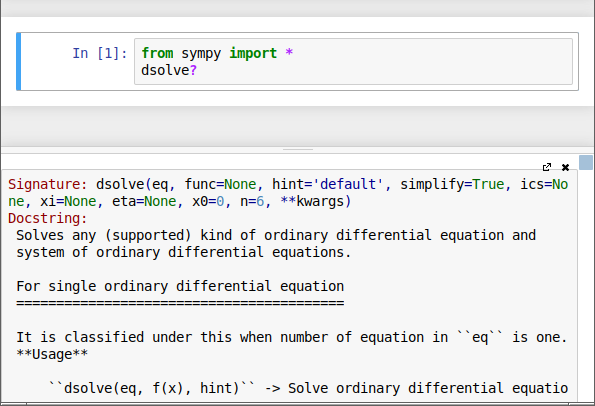
Also, if there's any doubt about the meaning or use of a keyword, one may type the keyword followed by a question mark to call up a help screen for that keyword:
Further Reading
There's much more to Jupyter than this introductory article has covered-- readers are encouraged to visit the official Jupyter documentation. Also, as mentioned earlier, Jupyter's sequel, named JupyterLab, is in rapid development and deserves exploration as well.
| Home | | Python | | | Share This Page |