Share This Page
| Home | | Editorial Opinion | | | | Share This Page |
An article in which I mourn the untimely passing of the example
All Content © Copyright 2012, Paul Lutus — Message Page
(double-click any word to see its definition)
Math ExampleEinstein once said, "If you can't explain it simply, you don't understand it well enough". This quote has a number of meanings that work at different levels:
- It argues that well-understood ideas should be amenable to simple explanation — and if not, maybe they aren't so well-understood after all.
- It recalls a time when people were willing to explain things to each other, seemingly a dying instinct.
- It suggests a time when descriptions were likely to include useful examples meant to turn the description into an educational opportunity for the listener.
In this article I explain (and lament) a decline in the quality of technical communications, in particular hardware and software documentation — a decline best demonstrated by the the disappearance of the example.
An example can take many forms:
- In computer programming, a short expository code sample showing how to use a new feature.
- For an idea in physics or nature, an equation, graph or animation that intuitively explains the idea.
- For virtually any field, a picture designed to clarify a point being made.
Lens ExampleFor example ... (see? — I practice what I preach) if I say "each member of the running sum of odd numbers is a perfect square," unless you're a mathematician, it's likely I will lose you, leave you confused. But if I include an example, especially in the form of a picture, you will almost certainly get it.
When I first heard this, I confess — I just didn't get it — I needed an ...Statement: Each member of the running sum of odd numbers is a perfect square.
Example:
Odd Number Count Running Sum Graphic Example 1 0 + 1 = 1
3 1 + 3 = 4
5 4 + 5 = 9
7 9 + 7 = 16
9 16 + 9 = 25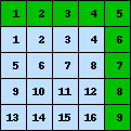
11 25 + 11 = 36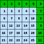
The picture shows things that words might not convey:
- A "perfect square" is a number whose square root is an integer — an integer that represents the width and height of a square.
- Each new number in the odd-number series fills the top and right sides of the old perfect square to make a new perfect square.
- Each new square construction requires an odd number.
- Each new odd number is able to build a new perfect square.
Readers may object that there are people who grasp ideas like this without needing a picture — they're called "mathematicians." Yes, that's true, but I ask — how many people might become decent mathematicians if only their brains can be trained with a few expository images, especially if the images take root in the rich soil of a young mind?
ProgrammingOne more example before we move on. When I was young I became interested in telescopes and astronomy. When I was 12 I struggled against big obstacles to acquire my own telescope. When I finally got my telescope, I spent many nights under the stars, looking at the moon, Mars, Jupiter. Then I began building my own telescopes — assembling lenses in various ways, but without any very useful results, for the simple reason that I had no idea how lenses worked — how they bent light.
I really wanted to know things like that, but I lived in an environment that celebrated mediocrity and ridiculed curiosity. I can remember being embarrassed even to speak up and ask about anything more complex than the location of a pencil sharpener.
Later, after I escaped from that environment, I learned something that any properly educated adult could have told me — lenses work by slowing light down. That's it — the big secret — the essence of lens optics. And I realized that an example, a picture, would have given me a key insight of immense value.
Well, all right, but at age 12 I couldn't really picture how that focused light beams. I needed an ...Statement: Lenses work by slowing light down.
Example: (click the image to run the animation)
= photons. (1) Snell's Law: $\displaystyle \frac{\sin \theta_1}{\sin \theta_2} = \frac{v_1}{v_2} = \frac{n_2}{n_1}$
Because photons take more time to pass through glass than air, the photons that pass through the edge of the lens arrive at the right sooner than those that pass through the thickest part of the lens. This is a simplified explanation for how a lens curves a light wavefront, and such a curved wavefront naturally converges to a point. Click here for a more complete explanation.
The near-perfect absence of examples in modern life has a deplorable effect — apart from making it difficult for people to acquire new skills, it replaces explanations with descriptions. By itself, a description is nearly useless. Here's a classic example:
- "The water suddenly receded from the beach" — just a description.
- "A sudden drop in water level is a warning sign of an approaching tsunami" — an explanation: run!
Now we will describe some cases where examples have seemingly disappeared, and explain why.
Java ExamplesAlthough it had its conceptual origins hundreds of years ago, computer programming is a relatively new activity and the field is in flux. New languages and techniques are announced almost daily, and some languages have embarrassingly short lives. This works against the crafting of useful examples.
Another factor in the erosion of the example are the automatic documentation features now embedded in some relatively new computer languages. Because a programmer can write a specially formatted comment at the top of each class and function, and because those comments will be automatically turned into a kind of documentation, for many people this ends any sense of responsibility to explain how the code works, or show how to apply it to practical problems.
Infamous Java GotchasJava tends to be a verbose language, and what should be a simple act like reading a file can sometimes be dauntingly complex. And the automatically generated documentation doesn't help. Here's a typical function that reads a file:
public String readFile(String filePath) {
  try {
    byte[] buffer = new byte[(int) new File(filePath).length()];
    BufferedInputStream f = new BufferedInputStream(new FileInputStream(filePath));
    f.read(buffer);
    f.close();
    return new String(buffer);
  }
  catch(Exception e) {
    System.out.println(e.toString());
  }
  return null;
}
About the above example, yes, contrary to what a student programmer may believe, in order to create a BufferedInputStream, you must first have a FileInputStream, and to use the BufferedInputStream, you must provide a buffer explicitly — this isn't done automatically. And Java programmers learn this by direct experience, it's not in the class documentation.
The idea of reading an entire file into a string for later manipulation is relatively new, and results from (a) a tremendous increase in a typical computer's memory size, and (b) more use of regular expressions to extract information from data, expressions that are easier to apply to a large amount of information at once.
Notwithstanding the above trend, in Java there's no self-evident, obvious, standard way to read a text file. Online resources basically show that it's a matter of opinion, and there are no concise approaches, only different, absurdly long methods like the above example. For contrast, here's a Python function that reads an entire text file:
def read_file(path):
  with open(path) as f:
    return f.read()
Some of Java's verbosity only reveals how old Java is, and how difficult it is to change a language after it's in use and must support a lot of legacy code. But without examples, things are much worse. A programmer who is unfamiliar with Java, and who reads the automatically generated documentation for File, FileInputStream and BufferedInputStream, is very unlikely to be able to figure out which elements to use, or assemble the elements into working code.
The great irony of Java is that, even though its programs are verbose, its documentation is spectacularly uninformative. Here's an example picked at random — the official documentation for BufferedInputStream — 1,500 words, and not one use example of any of the functions in the class. Because of this, programmers are reduced to going online and asking how to do things.
Android ExamplesNot to get into too much detail, but there are a couple of things about Java that defy common sense and that produce endless online inquiries from student programmers. One of them is string concatenation — essentially, appending one string onto another. In Java code it looks like this:
String s = "Now is the time";

s += " for all good men";

s +=  " to come to the aid";

s += " of their country.";

System.out.println(s);
String concatenation is a very common feature, all modern languages have it. But in Java, you don't want to do it in the way shown above. The reason is that, to append one string onto another, Java has to search for the end of the parent string, character by character, looking for its end mark (because Java doesn't store string lengths). As a string gets longer, this endless searching destroys the performance of the program, and for reasons that aren't obvious to a beginner. Best of all, the documentation for the String class mentions concatenation using '+', but mysteriously doesn't warn people not to do it.
In Java, the right way to build a string by concatenation is with the StringBuilder class — example.
The other infamous Java gotcha also involves strings — but this time it's string comparison. Most languages allow a simple way to compare two strings, and if the Java version actually worked, it would look like this:
boolean equalStrings(String a, String b) {
  // don't do this!
  return a == b;
}
The above code doesn't do what students think it does — it doesn't compare the characters in the strings, it simply compares the String objects for equality — is String object a the same object as b? This is a particularly nasty gotcha because it sometimes appears to be working (because for the sake of efficiency, identical strings may sometimes internally refer to a single string object). But then a case will come up in which two apparently identical strings will be separate String objects, and fail this comparison. The right way to compare strings for equality in java is:
boolean equalStrings(String a, String b) {
  return a.equals(b);
}
And do I need to mention that the official Java String class documentation doesn't mention this fact?
Readers may object that there are tutorials that cover these issues and they're relatively easy to find online. That's true, but it's also true that the first thing students read are the automatically generated class descriptions, which are spectacularly uninformative — "misleading" isn't too strong a word.
To those who read this and then ask, "so why use Java?" — although I agree with the sentiment, the fact is that Java runs practically anywhere, because Java programs run in a virtual machine, not native code. A Java virtual machine is available for most operating systems and platforms, so writing code in Java means your program will run nearly anywhere. And in my opinion, that's the only reason to write in Java.
MathematicsEvery force that ever conspired to produce well-ordered but useless documentation, and few useful examples, is at work in the Android operating system / platform created by Google. Most of the software is based on Java, so all the caveats and documentation issues from the above section apply to Android also.
As with Java, Android programmers search in vain for working examples, and as usual, the official documentation contains too few. With some notable exceptions, Android class descriptions describe every function in the class, but don't bother to either explain or provide examples.
To make things worse, there seems to be a gradual erosion in the open-source movement taking place — people who hope to make money from their Android applications are sometimes reluctant to publish their source code. What this means is that people end up reinventing the wheel, over and over, in separate, private struggles.
Android represents an abrupt jump in an otherwise smooth evolution toward languages and platforms that must function in diverse environments. Before the advent of Android and its many target devices, a computer program might need to take a few hardware and machine peculiarities into account — deviations from the standard target platform. But Android programs need to adjust themselves to accommodate anything between a high-end tablet computer with the resolution of a modern high-definition TV, down to a cellphone with a tiny display — and run the same on both. Add to this the periodic changes in Android itself, which sometimes break old programs.
There are Android code examples created by Google, but they're notoriously unreliable and often simply broken. Obviously these obstacles won't stop programmers committed to getting something out on the Android platform (including me) but this is true in spite of, not because of, the number of available working examples.
There may be a version of natural selection at work here — in my theory, once there are any code examples at all, Google's enthusiasm for creating more begins to decline, especially if something more economically productive presents itself, and for independent programmers, they first realize there aren't many useful code examples, then they ask a lot of questions and search the Web, they they acquire enough direct experience to create their own code examples. Obviously this model only benefits the public if the programmer accepts the open source model, a category that includes me:
- Source archive for CarpeTempus
- Source archive for SSHelper
- Source archive for SatfinderAndroid
- Source archive for TankCalcAndroid
In closing, I want to say that my criticism of Android is justly muted for the reason that Google did a reasonable job of documenting their code, and the number of examples (or the lack thereof) is hardly uncommon in modern times. And it seems the level of documentation hasn't stopped anyone willing to walk through fire to create an Android application.
Compound Interest ExampleMathematics is a perfect example of a skill that everyone needs but (in the U.S. at least) few understand. The list of reasons Americans don't understand mathematics is long, but one key reason is a lack of clear, useful examples — just as with programming.
The irony of innumeracy is that it begins at a time when the usefulness of mathematics isn't obvious (schools don't emphasize it enough), but the consequences last a lifetime after that — by not understanding mathematics, you give people the right to lie to you forever.
Compound People ExampleI can't think of a less appreciated and more powerful force in modern society than the various manifestations of compound interest (and compounding as an idea). It's a quick, efficient way to enslave incautious credit-card users, deceive house and car buyers, and drive a wedge between the rich and poor. About the last point, without appropriate public policies in place and if left unchecked, compound interest can destroy the middle class, leaving a society of very rich, very poor, and nothing between.
For example ... (an example I have used before but that bears repeating) let's say at the age of 20, John Doe inherits twenty thousand dollars. With a level of wisdom uncharacteristic for his age, John decides to deposit this inheritance in a long-term investment that returns 12% annually in interest compounded weekly. He intends to keep the investment account for 40 years until he's ready to retire at age 60. All that remains is to decide how to manage the account — leave it alone, or withdraw small amounts weekly?
Because of the effect of compound interest, the outcomes for various management choices may surprise most of my readers. Here are some outcomes from the above example (initial deposit $20,000.00, term 40 years, interest 12% per annum compounded weekly):
Option Account balance after 40 years Withdraw $46.00 per week $20,000.00 Withdraw $46.38 per week (0.8% more) $0.00 Withdraw $45.61 per week (0.8% less) $40,000.00 Forgo any withdrawals, let the account grow $2,416,852.17 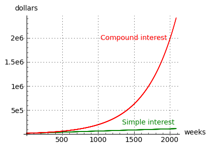 Figure 1: Simple/compound interest comparison
This result may shock some readers — if our wise investor withdraws 38 cents more per week, after 40 years he ends up with nothing. If he withdraws 39 cents less, he doubles his money. And if he forgoes the small weekly withdrawal, he ends up a millionaire. This example shows how compound interest can amplify seemingly unimportant choices or trends, in ways that most people don't appreciate.
Now to explain why this happens. Compound interest works by either charging or paying interest to an account, then deposits the result in the account, with the result that future interest transactions are performed on the account balance plus the prior accumulated interest. This is the reason for the amplifying effect. Figure 1 on this page compares outcomes for simple and compound interest, using the above problem's values and no weekly withdrawals.
Compound interest's tendency to amplify small differences over time explains why it has a destabilizing effect on society — because most people have bank accounts, mortgages, equities accounts, and credit card accounts, the behavior of interest-bearing accounts has a big impact on social stability and society's economic makeup over time. I've written a recent article on the economic aspects of this topic, so instead of making the same points here, I'll just link to it for further reading.
I also have a financial calculator page here that provides results and lists all the forms of the financial equations used in this section.
The basic idea is that nearly any process that builds on past results has this "compounding" behavior, and is prone to undermine people's expectations and "common sense" in some cases. The next example is population, a process that also "compounds".
Compounding Math ExplainedThe present world population growth rate is 1.1% per annum (births minus deaths, 2011). How long will it take for the population to double at that rate?
This example is simple enough that I will provide the equations used to compute population values — they're not very complicated and they should be usable on a hand calculator or a spreadsheet program. Here are the different forms of the equations that provide results for population (and other natural growth) problems:
(2) $ \displaystyle N = N_{0} \, e^{\left(r t\right)} $ (future population)
(3) $ \displaystyle N_0 = N \, e^{\left(-r t\right)} $ (present population)
(4) $ \displaystyle t = \frac{\log\left(\frac{N}{N_{0}}\right)}{r} $ (time)
(5) $ \displaystyle r = \frac{\log\left(\frac{N}{N_{0}}\right)}{t} $ (rate)
The variables are:
- N0 (initial population) = The population at time t = 0.
- N (future population) = The population at time t.
- r (rate) = The rate of population change as a function of t (a 1% increase is expressed as 0.01).
- This variable is called the Malthusian Parameter.
- In population studies, r is usually taken to mean births minus deaths.
- t (time) = The amount of time required to produce a growth in population proportional to N/N0.
- Note: "log()" in these equations refers to natural log, and e is the base of natural logarithms.
All right — now let's answer the above question: how long will it take to double world population, given the present growth rate of 1.1%? We want to use equation (4) above, and here is the result:
(6) $ \displaystyle t = \frac{\log\left(\frac{N}{N_{0}}\right)}{r} = \frac{\log\left(\frac{2}{1}\right)}{0.011} = 63.013 $ (years)This scary result is realistic only if the rate of population growth remains the same. And that result is realistic only if we don't change policies — educational, social, and medical.
Deriving Euler's NumberThe mathematics used to produce compounding results is surprisingly simple. Here is the equation used to acquire the future value of an annuity:
(7) $ \displaystyle fv = \frac{(1+ir)^n-1}{ir} pmt $Where:
- fv = future value.
- ir = periodic interest rate
- pmt = periodic payment
- n = number of compounding periods
This equation form only works for annuities that have an initial balance of zero, and in which the payment is made at the end of each period. But the point of this example is to show how this kind of equation works — by specifying how an annuity changes from one period to the next, and then multiplying this change by itself n times, with n representing the number of annuity periods.
For financial problems, the exponent n is assumed to be an integer (but this is not required), and the result is assumed to represent the outcome for a specific number of periods with fixed payments, and the process is assumed to represent a series of incremental jumps. For many other problems, these assumption are not present, and a smoother, more continuous relationship is assumed to exist, for example between time and changes in a large population of organisms that have the previously described "compounding" property. It is for problems like this that a special constant exists. The constant, identified by the letter e, uniquely represents natural growth processes. Let's try to derive it.
Differential Equation Example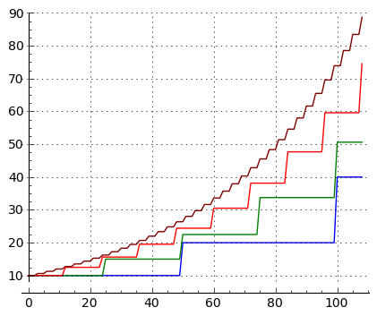 Figure 2: Effect of step size on growth pattern
Let's say we want to represent an increase in a quantity Q. The increase ratio is represented by r, and we perform a stepwise increase like this:
(8) $ Q_{n+1} = Q_{n} (1+r) $Using this approach, a 10% increase in Q might be represented this way:
(9) $ Q_{n+1} = Q_{n} (1+.1) $The above method may be suitable for a single abrupt increase of (for example) 10%, but isn't suitable for a gradual growth process more typical of natural processes like bacterial colony growth. How shall we make our procedure more closely resemble nature? Well, we can apply the desired increase ratio r in more steps, like this:
(10) $ Q_{n+1} = Q_{n} (1+\frac{r}{n})^n $In this formulation, if n = 1, the outcome is the same as before, an abrupt increase. But if we increase the value of n, there are more increments, each with a smaller percentage increase, as shown in Figure 2. The trend shown in Figure 2, between the blue (coarse) trace and the brown (nearly smooth) trace, more closely imitates a natural process with either many small increments of change, or a large measured population, or both.
Figure 2 tells us that a large number of steps (a large value for n) more closely approximates a natural process of growth. Let's see if we can further improve this process and arrive at a value that can be used instead of equation (10) and similar equations. Here is a version of equation (10) that we can use to test different n values and the results:
(11) $ Q = (1+\frac{1}{n})^n $Here is a table with results from equation (11) for increasing values of n:
n Q 1 2.00000000 10 2.59374246 100 2.70481383 1000 2.71692393 10000 2.71814593 100000 2.71826824 1000000 2.71828047 10000000 2.71828169 100000000 2.71828180 1000000000 2.71828205 In the table above we obtain an estimate for a numerical constant that seems to simulate natural growth processes, and that can be used to produce results that might otherwise requires an infinite number of infinitesimally small steps if they had to be computed as we have been doing. Here is the formal definition for e, which is known as Euler's Number:
(12) $ \displaystyle e = \lim_{n \rightarrow \infty} (1+\frac{1}{n})^n$For those unfamiliar with Calculus notation, the above means "as n approaches infinity, e approaches the value of Euler's Number."
Electronic R-C Circuit ExampleAbove we explored a function that modeled the growth of a natural system whose future growth depended on its past growth, in other words, its rate of change was self-referential. Such processes are obvious applications for expressions that rely on Euler's number e.
There is another large class of natural processes with a different kind of self-referential property — systems where the rate of change depends on the remaining distance to be covered. Here are some examples:
- Two objects at different temperatures, exchanging heat energy.
- Two bodies of water at different heights, exchanging water.
- Two gas reservoirs at different pressures, exchanging gas.
- An electronic resistor-capacitor circuit where the capacitor's voltage differs from the source voltage.
- A radioactive isotope undergoing natural decay.
- Many others.
In all these cases, the rate of change in a measured quantity (temperature, gas pressure, water height, voltage, decay rate) is proportional to the remaining distance.
Before I show examples of these functions, I would like to digress into the mathematical method one uses to create them — differential equations.
A differential equation is much like an ordinary algebraic equation, except that it contains one or more derivatives, or statements about rates of change.
For example, we might say, about an unknown function f(t):
- $ \displaystyle f(t) + \frac{f'(t)}{k} - b = 0$
- $ \displaystyle f(0) = a$
Where:
- t = time
- f(t) = the unknown function
- f'(t) = the rate of change in the function with respect to time (note the apostrophe)
- a = initial value
- b = ending value
- k = rate-of-change constant
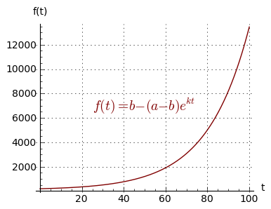 Figure 3: Example growth function
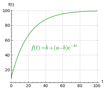 Figure 4: Example decay function
Let's explain the above statements in plain language:
- "$f(t) + \frac{f'(t)}{k} - b = 0$" means the function's value, plus its rate of change divided by k, is equal to b. This means that, as time passes, the function's value will move toward b, but because the value is increasing, the rate of change must therefore decrease, because their sum is equal to b, the end value.
- "f(0) = a" simply means the function's initial value (at time zero) is equal to a, the start value.
It seems I have described a function that has an initial value of a at time zero, and that will show a relatively large rate of change at first, but because the sum of the function and its rate of change is equal to the end point b, the rate at which the function approaches b should decline — in fact, if you think about it, because the rate of change represents the difference between the function and b, the function should never quite equal b.
In the next step, we will identify the unknown function.
Digression: As enthusiastic as I am about differential equations and their many practical uses, I won't be offering a technical summary of how one converts differential terms like those above into a function that matches the terms. Instead, below I will suggest ways to get a result without actually having to learn these methods in depth. And my reason is simple — I think people should be allowed to see some of the power of mathematics before having to tackle the difficult parts. If this idea has value (and I think it does), it suggests that most of present-day math education is upside-down — long division with paper and pencil before pretty pictures. End of digression.
Here are some resources the reader may want to use to acquire results like this one:
- Sage, a free, open-source mathematics resource that is able to solve this class of differential equation. Here are the Sage entries that solve this differential equation:
var('t k a b')And here is Sage's output:
y = function('y',t)
f(t) = b + desolve(y + diff(y,t)/k == 0,[y,t],ics=[0,a-b])$ \displaystyle f(t) = {\left(a - b\right)} e^{\left(-k t\right)} + b $- Wolfram Alpha. If I submit "f(t) + f'(t)/k - b = 0,f(0) = a" to Wolfram Alpha, I get this result (one must click "Show Steps" to get it in the displayed form):
$ \displaystyle f(t) = b + (a-b)e^{-kt} $- Mathematica can solve this equation also. Here is a Mathematica entry that produces a solution:
DSolve[{f[t] + f'[t] k - b == 0, f[0] == a}, f[t], t]Unfortunately, it turns out that Mathematics 5's result, which agrees with the above solutions, can't be exported into the mortal world. And, since Sage is free and can do much of what Mathematica does, I'm not planning to "upgrade" Mathematica.
- There are many other resources for this kind of processing, and there's always the option of learning enough mathematics to be able to produce this kind of result directly (example resource).
Figures 3 and 4 show two forms of this equation, one for exponential growth, the other for exponential decay. To provide a bit more detail, the two sets of differential terms are:
Growth equation:
Terms:
- $ \displaystyle f(t) - \frac{f'(t)}{k} - b = 0$
- $ \displaystyle f(0) = a$
Resulting equation:
(13) $ \displaystyle f(t) = b - (a-b)e^{kt} $Decay equation:
Terms:
- $ \displaystyle f(t) + \frac{f'(t)}{k} - b = 0$
- $ \displaystyle f(0) = a$
Resulting Equation:
(14) $ \displaystyle f(t) = b + (a-b)e^{-kt} $The above comparison is more to show how simple it is to acquire equations with unrelated purposes by changing one character in a differential term, than it is to produce two equally useful equation forms — the exponential growth form doesn't limit itself to the boundaries set up by variables a and b.
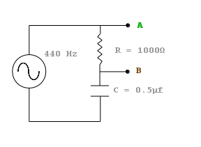
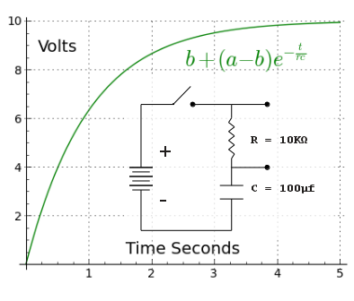 Figure 5: Resistor-capacitor circuit
Periodic Waveform Circuit ExampleBecause of their self-referential property, equations (13) and (14) find very wide application in physics and related fields. As discussed earlier, they can be used to model a remarkable number of physical systems in many fields. Let's use an electronic R-C (resistor-capacitor) circuit as an example.
A capacitor is in essence an analog current integrator — in an R-C circuit, the voltage on the capacitor is the integral of applied currents with respect to time.
- In the example problem shown in Figure 5, a switch is closed at time zero, and current begins to flow through the resistor.
- The circuit current causes the capacitor to begin charging — its voltage increases.
- Because the voltage on the capacitor is increasing, the voltage across the resistor is decreasing.
- As the resistor's voltage decreases, so does the current in the circuit (because $I = \frac{E}{R}$).
- Because the circuit current is decreasing, the capacitor's rate of charge also decreases.
- This self-referential relationship between resistor and capacitor creates an exact parallel with the original differential terms for the equation being used: the capacitor plays the part of f(t), the quantity, and the resistor plays the part of f'(t), the rate of change in quantity.
- It's important to understand that, because of the nature of this circuit and its mathematics, the capacitor never gets to the source voltage. This is true for all equations that use Euler's Number e to model natural processes with a negative exponent — over time they approach but do not equal the limit represented by variable b in this example. In mathematics this is called an asymptote — a goal approached but never reached.
With this example, my purpose has been to show that mathematics has practical applications, that many everyday devices can be modeled with arbitrary precision using equations, and that the relationship between mathematical terms and physical devices is sometimes very clear.
Orbital Mechanics ExampleIn the above example we analyzed a differential equation that models a decaying process, a system in which a function's rate of change depends on a difference between levels. That analysis only works for fixed levels, but in the real world of electronic circuits, we're more likely to encounter periodic waveforms. Let's see if we can write a differential equation like the above, but one that works with a periodic waveform. Here is a differential term that describes the function we need:
(15) $ \displaystyle y(t) + y'(t) \, k = \sin(\omega t) $
Figure 6: Sinewave Circuit Diagram
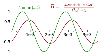
Figure 7: Sinewave Circuit Graph
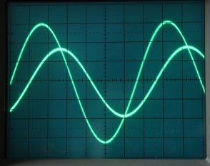
Figure 8: Sinewave Circuit Oscilloscope Image
In the earlier differential equation examples, we set initial and final values, for example to move between levels a and b. But because this is a periodic process, it doesn't require an initial value, so the complete description for this differential equation is a single term.
Here are Sage entries that produce a solution for the above expression:
y = function('y',t)
de = y + k*diff(y,t) == sin(omega * t)
des = desolve(de,[y,t])Notes:
- In the above code, omega (ω) is a convenience variable that is equal to $2 \pi f$, f = frequency in Hertz.
- k is another convenience variable that stands in for R × C in a very familiar-looking resistor-capacitor circuit shown in Figure 6.
- These stand-in variables are meant to simplify interpretation as equations become more complex.
Here is Sage's solution:
(16) $ {\left(c - \frac{{\left(\omega \cos\left(\omega t\right) - \frac{\sin\left(\omega t\right)}{k}\right)} e^{\frac{t}{k}}}{{\left(\frac{1}{k^{2}} + \omega^{2}\right)} k}\right)} e^{\left(-\frac{t}{k}\right)} $Without getting into too much technical detail, equation (16) is Sage's way of honoring the need for a constant c that must be taken into account when we write an indefinite integral. Unfortunately the presence of c greatly complicates the result, and because this is a periodic function based on the sine function whose average value is zero, we can and should set c to zero. Here's the Sage entry that does this, while assigning the outcome to a function:
sf(t,k,omega) =
des.subs(c = 0).full_simplify()And our result sinewave function is:
(17) $ \displaystyle sf(t,k,\omega) = -\frac{k \omega \cos\left(\omega t\right) - \sin\left(\omega t\right)}{k^{2} \omega^{2} + 1} $Figure 7, a graph for equation (17), compares the signal source waveform located at point A to the capacitor waveform located at point B of figure 6. And Figure 8 shows an oscilloscope image — a result from "reality" — displaying the same A/B comparison as in Figure 7, but using actual electronic components and a signal generator.
Before we move on, I ask my readers to think about what is being shown in figures 7 and 8. Remember that the A waveform is a sinewave reference signal being provided to an R-C circuit, and the B waveform shows the resulting capacitor voltage. If we think about the capacitor's role, we realize that its voltage represents the time integral of the applied waveform, and therefore when the source waveform's voltage is equal to the capacitor's voltage, there should be no current flowing and the capacitor's voltage should stop changing. And that's exactly what we see — when the A voltage equals the B voltage (when the A trace crosses the B trace), the function's first derivative is equal to zero and the capacitor's voltage shows an inflection point.
Computing an OrbitOver the years I've written many orbital simulations and they've gradually become better and more efficient (1,2,3). In this example I will describe the most recent of these simulations, which is computationally more efficient, works in three spatial dimensions, is able to compute the behavior of many simultaneous objects, and supports true 3D viewing as well. Let's start with a review of gravity's properties:
- There are four fundamental forces in nature. In order of their strength, they are the strong, electromagnetic, weak and gravitational.
- The gravitational force, though the weakest, has infinite range. Its carrier particle (in the incomplete quantum theory of gravity) is the graviton, and its force declines as the square of distance.
- Matter that has mass, also has two properties relevant to this discussion: attraction to other masses, and inertia.
- A larger mass has a proportionally larger attraction to other masses, but it also has proportionally more inertia. This leads to the Equivalence Principle, the idea that gravitational and inertial mass are equal.
- Consistent with item (4) above, in the case of a small object attracted to a large object, if the large object is much more massive than the small, the mass of the small object may sometimes be disregarded in calculations, on the ground that the small object's gravitational attraction is moderated by its inertia, making its behavior essentially equal to other objects in its size range (imagine Galileo Galilei dropping different-sized weights from the Leaning Tower of Pisa.
- With respect to gravitationally orbiting bodies, analytical solutions are available for two bodies, but all cases involving more than two bodies must be solved numerically (three-body problem).
- Because of the limitation described in item (6) above, all orbital simulations except the most trivial are performed numerically, usually with computer programs like that described in this example.
- An object in orbit, absent friction, maintains the same total energy, regardless of how much its velocity changes during its orbit. An object does this by exchanging potential and kinetic energy — high kinetic energy at periapsis, high potential energy at apoapsis, but the two energies always sum to a constant. This interesting result is easily obtained from a simple orbital simulation, and confirms the important role played by energy conservation in orbital mechanics.
Okay, having set the stage, let's now look at the mathematics of orbital simulation. We begin with the gravitational force equation:
(18) $ \displaystyle f = G \frac{m_1 m_2}{r^2} $Where:
- f = Force between masses $m_1$ and $m_2$, with units of newtons.
- G = The universal gravitational constant, with the approximate value 6.67384 x 10⁻¹¹ N m2 kg-2.
- $m_1,m_2$ = Two masses in mutual attraction, units kilograms.
- r = distance between $m_1$ and $m_2$, meters.
In principle, every gravitational computation could be performed using equation (18). But for applications near the earth's surface, a simpler equation can be derived that includes some assumptions:
- That the objects being modeled have masses much smaller than earth's mass, meaning the Equivalence Principle makes them essentially equal.
- That the values obtained apply to locations near the earth's surface.
Given the limitations above, and with these values:
- $e_m$ = Earth's mass: 5.9736 × 1024 kilograms.
- $e_r$ = Earth's radius: 6.371 × 10⁶ meters.
- $G$ = Described above.
We can compute a gravitational acceleration of:
(19) $\displaystyle g = G \frac{e_m}{e_r^2} = 9.82257 \frac{m}{s^2} $ for small masses.The above quantity, called "little-g," is widely used for gravitational calculations near the earth's surface.
Python Orbit Simulation ExampleTo compute the orbit of mass m2 around mass m1, one numerically solves a differential equation repeatedly. For each position update, we need the following elements:
- A scalar distance r between masses m1 and m2, which in three dimensions is equal to:
(20) $ \displaystyle r = \sqrt{(m_1 x-m_2 x)^2 + (m_1 y-m_2 y)^2 + (m_1 z-m_2 z)^2} $A unit vector $\hat{r}$ that provides a direction for accelerations and velocities. A unit vector has a magnitude of 1, which means it can be used as a term in equations where only a direction for a force or velocity are required.
For two objects having a relative angle of θ, an example two-dimensional unit vector would be equal to:
(21) $ \displaystyle \hat{r} = \{ \cos \theta , \sin \theta \} $A force vector $\vec{f}$, which represents a computation of the gravitational inverse square law as a scalar, times a unit vector $\hat{r}$ that provides a direction for the force:
(22) $ \displaystyle \vec{f} = \frac{-G m_1 m_2}{r^2} \hat{r} $Where:
- $\vec{f}$ = a force vector, units Newtons, that attracts m1 and m2.
- r = from equation (20) above.
- $\hat{r}$ = unit vector from equation (21) above.
- A velocity vector $\vec{v}$. As an example of an initial velocity value, a circular orbit requires:
(23) $ \displaystyle \vec{v} = \sqrt{\frac{GM}{r}}\hat{r} $Where:
- G = universal gravitational constant, discussed earlier.
- M = the mass of the larger of the two bodies, with the understanding that the orbiting mass is much smaller than the mass represented by M.
- $\vec{v}$ = velocity vector, which for a circular orbit is initially directed perpendicular to the unit vector $\hat{r}$.
- r = from equation (20) above.
- $\hat{r}$ = unit vector from equation (21) above.
As the simulation proceeds, the velocity vector is updated using the force vector from equation (22).
With the above quantities, one can accurately model an orbit by selecting an appropriate time interval Δt and repeating these steps:
- Use equation (20) to compute the scalar distance r between m1 and m2.
- Use equation (21) to compute a unit vector $\hat{r}$ based on the relative position of m1 and m2.
- Use equation (22) to compute a directed gravitational force.
- Use an equation like (23) above to set an initial velocity at time zero, then as the simulation proceeds, update the velocity using the result from equation (22).
- Using the currently computed velocity vector, update the position of the modeled body and use the result.
- Repeat the process from step (1) above.
When experimenting with orbital computation, several things become apparent. One, to speed things up one might want to use a large Δt (a large step size of simulated time), but this can cause unacceptable numerical errors. Orbital simulation is a tradeoff between high accuracy and fast program execution. Two, there are many possible code optimizations, the effectiveness of which sometimes depends on the language in use, whether or not the program is compiled, and how many processors are available.
Over a period of years I have experimented with ways to reduce the complexity of three-dimensional orbital force and velocity calculations. I started out simply computing a unit vector as shown above in equation (21), but that is the least efficient approach, and in three dimensions it's even less efficient. My thinking on this topic (and my code) has evolved like this:
- Initially, I computed a force vector that combined equations (21) and (22) above, which required a square root and two trigonometric results.
- Then it occurred to me that, because I had computed r in equation (20), I in essence had the hypotenuse of a right triangle, and I could combine the hypotenuse with the position values to derive the sin θ and cos θ values for my unit vector without having to call trigonometric functions.
- At that stage I was computing an inverse square (scalar) force, then multiplying it by my unit vector to produce a force vector. To put this another way, I needed the hypotenuse for my unit vector, and that meant computing a square root, but for the inverse square calculation, I only needed the sum of the squares of the distances.
I then discovered that I could combine the operations of (a) inverse square gravitational attraction and (b) unit vector computation. I found I could take my previously computed hypotenuse, multiply it by the position vector to get a unit vector, then multiply by an inverse cube to (a) normalize the position value and (b) accomplish the inverse square part of the computation. At that stage my velocity computation looked like this:
(24) $ \displaystyle \vec{v_{n+1}} = \vec{v_{n}} + \vec{p} \, \sqrt{x^2+y^2+z^2}^{-3} $ (p = position)Within a short time I realized that equation (24) could be optimized to:
(25) $ \displaystyle \vec{p} \, \sqrt{x^2+y^2+z^2}^{-3} = \vec{p} \, (x^2+y^2+z^2)^{-3/2} $- Overall I had eliminated a square root computation and two trigonometric computations. In its final form, this method has a number of adds and multiplies and a single power computation, and is much more efficient.
JavaScript Orbit Simulation ExampleHere is a Python program listing that performs a 2D orbital simulation using the methods described above (click here for plain-text):
import sys, math

# universal gravitational constant
G = 6.67428e-11

# earth mass
e_mass = 5.9736e+024

orbit_radius = 8.0e7

# circular orbit velocity
cov = math.sqrt(G * e_mass / orbit_radius)

# position
pos = complex(orbit_radius,0)

# velocity: set elliptical orbit: cov/3
vel = complex(0,cov)/3

dt = .1 # delta-t seconds

n = 0

# energy max and min
emax = -1e9
emin = 1e9

# simulate orbit

while True:
  # update velocity
  vel += pos * -G * e_mass * dt * abs(pos)**-3
  # update position
  pos += vel * dt
  # get magnitudes
  r = abs(pos)
  v = abs(vel)
  # calculate total energy: KE + PE
  e = (v**2)/2 -(G * e_mass / r)
  # collect min and max energy bounds
  emax = max(emax,e)
  emin = min(emin,e)
  # compute error
  error = abs((emax-emin) * 100 / emin)
  # display results
  # show only a few results
  if(n % 10000 == 0):
    print 'p = %8.4e v = %8.4e e = %8.4e error = %6.2e%%' % (r,v,e,error)
  n += 1
The Python orbital simulation above is shorter than it would be in most languages, for a couple of reasons — one, Python naturally tends to be concise, and two, Python supports complex numbers, which greatly reduces the amount of code required to support a 2D orbital simulation.
Those who run the above script will see that the sum of kinetic and potential energy is approximately constant. In this simulation the error is less than 1% over time, showing that the algorithm is a reasonably accurate simulation of reality (it can be made more accurate by reducing the time step dt, but that requires a longer running time).
Let me explain how the above energy measurement validates the accuracy of an orbital simulation. The degree to which a simulation reflects reality can be tested -- all one needs to do is measure the total energy (the sum of kinetic and potential energy) in an elliptical orbit, and see how much it varies over time. In nature, the sum of kinetic and potential energy should not change at all during an orbit -- all one should see is a periodic conversion from kinetic to potential energy and the reverse, depending on the object's position in the orbit, but to agree with the principle of energy conservation, the two energy values should sum to a constant.
Orbital mechanics recognizes and incorporates the idea of energy conservation. In an elliptical orbit, an object can have a great number of distances from the parent body, and a great number of orbital velocities. The radius parameter represents gravitational potential energy, and the velocity parameter represents kinetic energy. If energy is conserved, the two kinds of energy should sum to a constant at any point in the orbit:
Gravitational potential energy:
(26) $ \displaystyle PE = -\frac{G M m}{r} $ (27) $ \displaystyle KE = \frac{m v^2}{2} $Total energy (should be constant during an orbit):
(28) $ \displaystyle E = \frac{m v^2}{2} -\frac{GMm}{r} $It turns out that, in a deep sense, this modern requirement that the two kinds of orbital energy must sum to a constant, and Kepler's Second Law of orbital motion (an object sweeps out equal areas in equal times), both mean the same thing. Click here to see these issues explored in greater depth.
The orbital simulator below is by far the most advanced I have written, but is in some technical ways the simplest (for reasons given above). It uses the new HTML5 "Canvas" feature to allow easier display than many of my prior programs, most of which used a Java applet for display.
In testing I have found that older Microsoft browsers either don't support the industry standard features required for this display, or they run very slowly and make errors. If you have difficulty using this simulator with your Microsoft browser, I recommend that you use a different browser — any other browser. Download Firefox here. Download Google Chrome here.
To start and stop the simulation, click the display below. And to fully appreciate the impact of this 3D orbital simulation, you really should get hold of some anaglyphic glasses (
) and view it in 3D. When you're ready for a deep experience, just click the "anaglyphic" selector below. To get more or fewer comets, just type a number at the "Comets" entry window.
(Click display to start/stop animation)
Comets:
| Home | | Editorial Opinion | | | | Share This Page |