3. The Fast Fourier Transform

The most common form of the Fast Fourier Transform (FFT) can be credited to Carl Friedrich Gauss, who created it as a method to evaluate the orbits of the asteroids Pallas and Juno around 1805. Unfortunately, and not unlike Isaac Newton, Gauss published his result without also publishing his method (it was only published posthumously). Variations on this method were reinvented during the 19th and 20th centuries, but credit is often given to J.W. Cooley and John Tukey, who in 1965 published an FFT embodiment now known as the Cooley-Tukey Algorithm, meant for automatic computation.

The basic idea of the Cooley-Tukey algorithm (of which there are many variations) is to improve the efficiency of the Discrete Fourier Transform (DFT) by dividing the computation into subunits. For the DFT, efficiency can be improved by recursively dividing a DFT of size N into two interleaved DFTs of size N/2 (and that consequently requires the data set size to be a power of 2). A practical embodiment converts an algorithm requiring O(n²) time to one only requiring O(N log N) time.

A full explanation of the FFT is beyond the scope of this article, but there are excellent online references to provide more depth, also see the reference list at the bottom of this page.

One of the ironies of the FFT is that it was originally created to allow manual computations that would have been utterly impractical, but in the modern era of very fast computers, the FFT is now regarded as essential to producing results fast enough to meet our jaded expectations.

The source code package that accompanies this article contains a highly optimized C++ embodiment of the Cooley-Tukey algorithm, plus a number of ancillary programs for creating data and for plotting the results. Here are instructions for using the programs:

The source code package assumes a system running Linux. Those running Windows may be able to adapt the code to that platform's requirements, or they can install Cygwin, a valiant method to graft some of Linux onto Windows. Or they can install Linux. The last method is to be preferred.
To install the source code package:

Make sure you have a C++ compiler installed: "yum install gcc" or "apt-get install gcc".
Make sure you have gnuplot installed: "yum install gnuplot" or "apt-get install gnuplot" (gnuplot is used to graph the results).
Download this tar archive to your system and place it in any convenient directory.
Open a shell session in the download directory and perform these steps:
$ tar -xzf signal_processing.tar.gz
$ make
Barring any errors, several executable files will appear in the target directory (click the names to see the corresponding source code listing):
- fft_processor (performs FFT and IFFT conversions)
- gnuplot_driver (provides gnuplot with plotting information)
- signal_source (creates a sample waveform and optional noise)
- sound_source (creates a data stream from a real-time sound source such as a microphone)

Now we can use the FFT to produce some results:

Open a shell session in the target directory and perform this preliminary test:

$ ./signal_source -a 2048 -s 400 -f 100 -m 50 -n 3 | ./fft_processor | ./gnuplot_driver -p

(You should be able to copy these examples from your browser into your shell session, but don't copy the '$' character, it is present only to remind you that it's a shell session.)
If all is well, this result will appear:

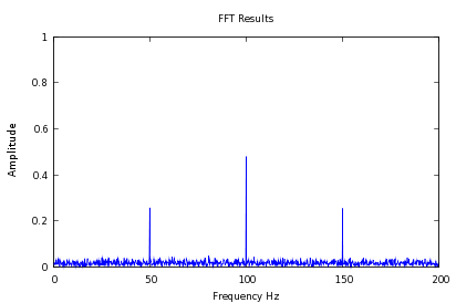
(For a touch of realism I have intentionally introduced some noise into these examples.)

Next, we create an animated real-time conversion of the above example (type Ctrl+C to stop it):

$ ./signal_source -a 2048 -s 400 -f 100 -m 50 -n 3 -c | ./fft_processor | ./gnuplot_driver
Now we'll create an animated plot of the source signal, before conversion to the frequency domain (type Ctrl+C to stop it):

$ ./signal_source -a 2048 -s 10000 -f 100 -m 10 -n 1 -c | ./gnuplot_driver -i

This is what the result should look like:
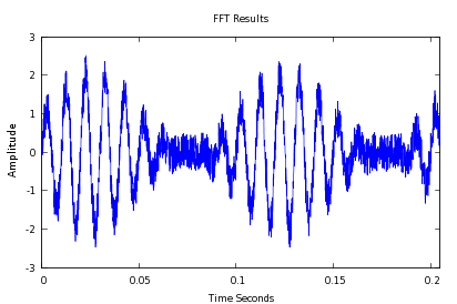
The display speed of the animated examples is limited primarily by the time required to plot the results, not to convert from the time to frequency domains.
Here is an example where a signal is plotted, then the signal is converted to the frequency domain, then reconverted back to the time domain to be plotted and compared to the original:
1. Plot the original signal:
  $ ./signal_source -a 2048 -s 10000 -f 100 -m 10 -n 0 | ./gnuplot_driver -i -p
2. Convert to the frequency domain, reconvert back to time domain, and plot the result:
  $ ./signal_source -a 2048 -s 10000 -f 100 -m 10 -n 0 | ./fft_processor | ./fft_processor -i | ./gnuplot_driver -i -p
Notice about the above example that the second invocation of the FFT processor has the command-line argument "-i" meaning "inverse".

Here is an example that uses a sound source like a microphone rather than a signal generator, and creates an animated spectral display of room sounds. It is the least reliable example because of differences between systems, and may require some experimentation to get it to work.
- I have a Webcam attached to my system, the Webcam has a microphone, and I know the sound source for this input is /dev/dsp1. So on my system, I can get an animated sound spectrum with this entry:
  
  $ ./sound_source -i /dev/dsp1 -a 512 -s 4000 | ./fft_processor | ./gnuplot_driver
- Here is a sample frame from the resulting animation (the conspicuous signal was created with a 440 Hz tuning fork):
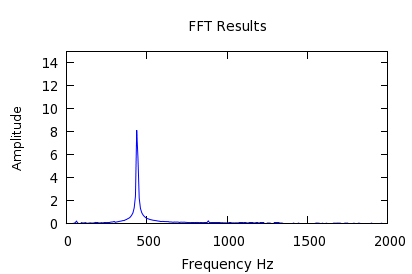
- Capturing sounds from a sound card in real time is fraught with difficulties. Most of the time is spent waiting for input, rather than converting to a spectrum with the FFT or plotting.

The sample programs have been designed to maximize flexibility and encourage experimentation, and are being released in response to the many requests by educators since the release of my earlier project FFTExplorer. All the programs are released under the GPL, so they can be used in your own projects. Here are some details:

Each of the sample programs will print its command-line options if invoked with "program_name -h".
All the sample programs use a common stream data format, to allow them to be piped in various ways. Here is an explanation.
- Run this example to see the output:
  
  $ ./signal_source -a 8 -s 4 -f 1 -m 0 -n 0
- This entry means an array size of 8, 4 samples per second, a frequency of 1 Hz, a modulation frequency of 0, and a noise level of 0.
- Here is the output:
```
8
4
0 0
1 0
1.22461e-16 0
-1 0
-2.44921e-16 0
1 0
3.67382e-16 0
-1 0
                    
```
- The data stream has this definition — each component appears on a separate line:
  - The array size.
  - The sampling rate in samples per second.
  - Complex data pairs equal in number to the array size, with real and imaginary parts separated by a space.
- The program responsible for creating the signal defines the array size and the sampling rate. The remaining programs in the chain simply pass these values along with modified data. The FFT program uses the array size to govern its conversion activities, and the gnuplot driver uses both the array size and the sampling rate to produce meaningful graph indices.
The above-described data stream format is designed to simplify experimentation and entails some sacrifice of speed. Real-world applications of the FFT don't normally use this method, instead they integrate signal sources and FFT conversions into a single program.

Here is a listing of source file names, linked to the respective source files, plus comments. Remember that all the sources, plus a makefile, are available more conveniently in this tar archive.

Core Processing Routines
- Complex.cpp, Complex.h
  
  A complex number class meant to simplify the handling of complex numbers, at some expense of execution speed.
- DFT.cpp, DFT.h
  
  A Discrete Fourier Transform routine, included for its simplicity and educational value. Very slow. Users can invoke this conversion with "$ ./fft_processor -d".
- FFT.cpp, FFT.h
  
  A well-optimized Fast Fourier Transform using the Danielson-Lanzcos lemma. This routine, like most in its class, requires that the array size be a power of 2. Notice that an array of bit-reversed pointers is created in advance of computation, an optimization that pays off during multiple conversions using the same array size (for a single conversion it has no effect).
  
  Readers familiar with FFT code examples may be surprised by the relative brevity of the main conversion routine. This results from use of a Complex number class (see above) that handles some operations in a way that allows a simplification of the source, probably at the expense of execution speed. There are faster FFT routines available (example: FFTW), but they tend to be unreadable and therefore unmodifiable.
Utility and Example Programs
- Most of these programs will display their options if invoked like this: "$ program_name -h".
- fft_processor.cpp
  This program acts as an interface between the data stream and the core FFT/DFT routines. Most of its operational parameters are determined by the signal source (see below).
  
  Here are the command-line options:
```
Usage: [-i (inverse FFT/DFT)]
       [-d (DFT instead of FFT)]
                      
```
- gnuplot_driver.cpp
  This program processes the stream data for presentation to the gnuplot plotting program. It has quite a number of options. Pay particular attention to the "-i" option, which is meant to mirror the fft_processor "-i" option, e.g. when a time-domain signal is being displayed, use this program's "-i" option so the horizontal axis has units of time instead of frequency.
  
  Here are the command-line options:
```
Usage: [-i(nverse mode)]
       [-t (chart title, default "FFT Results"]
       [-x (x axis title, default "Frequency Hz")]
       [-y (y axis title, default "Amplitude")]
       [-r (raise)]
       [-p (persist)]
       [-c (trace color, default "blue")]
       [-b (background color, default "white")]
                      
```
  NOTE: At the time of writing, the current version of gnuplot (4.2 patchlevel 3) doesn't allow its background color to be changed. This may change in the future, and it was not true in earlier builds.
- mulaw_converter.cpp, mulaw_converter.h
  
  A utility routine that allows the "sound_source" program to support Mu-Law sound sources.
- signal_source.cpp
  This program generates a number of different signals, but primarily a classic modulated AM radio wave. The user may add some noise for realism during animations and for other purposes.
  
  This program can be looked on as a prototype for any special-purpose signal generators the reader may wish to create, by modifying the core generation routine to suit personal preferences.
  
  Here are the command-line options:
```
Usage: [-a(rray_size, must be a power of 2, default 2048)]
       [-s(amples_per_second, default 1000)]
       [-c(ontinuous)]
       [-f carrier freq, default 100] [-m modulation freq default 10]
       [-n noise level, default 0.3]
                      
```
- sound_source.cpp
  This program allows use of a sound-card signal source. It is the most Linux-specific of the example programs, and even on a Linux system it will require some experimentation to sort out its operation.
  
  Here are the command-line options:
```
Usage: [-i(nput, default /dev/dsp)]
       [-f(ormat: 0=unsigned 16-bit, 1=signed 16-bit, 2=muLaw, default 0)]
       [-a(rray_size, must be a power of 2, default 2048)]
       [-s(amples_per_second, default 1000)]
                      
```