

 Share This Page
| Home | | Mathematics | | * Sage | | | | Share This Page |
Applying Sage to finance
— P. Lutus — Message Page — Copyright © 2009, P. Lutus(double-click any word to see its definition)
To navigate this multi-page article:Use the drop-down lists and arrow icons located at the top and bottom of each page.
Click here to download a copy of the
Sage worksheet used in preparation of this article.
This article shows how Sage can take a single function with multiple arguments and create a related set of functions, each returning one of the original arguments as a result. The key function computes the future value (fv) of a compound-interest annuity with a fixed interest rate. The future value equation system uses the following arguments to compute its results (in the complete equation system, each of these values appears either as an argument or as part of a function name):
- fv = future value of an investment (capitalization)
- pv = present value of an investment (discounting)
- pmt = payment per period
- ir = interest rate per period
- np = number of periods
- pb = flag: payment at beginning (1) or end (0)
Some notes on these variables and the equations they work with:
- The interest rate is per period — if a loan has a 12% annual interest rate, and the payments are monthly, the interest rate is 1%.
- The interest rate is expressed as a value, not a percentage — 1% is expressed as 0.01.
- Payments into the account and adverse interest rates are negative numbers, payments out of the account and interest rates in the investor's favor are positive numbers.
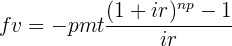
The simplest expression for a future value calculation is very simple indeed:
Let's put the above equation into Sage. But first, as with prior articles in this set, let's create a worksheet cell with some convenient initializations (readers may also download this article's
#auto
reset()
forget()
# special equation rendering
def render(x,name = "temp.png",size = "normal"):
    if(type(x) != type("")): x = latex(x)
    latex.eval("\\" + size + " $" + x + "$",{},"",name)
import re
# format latex with spaces between multi-character names
def latex_spc(x):
    r = latex(x)
    return "$" + re.sub("(\{\w+\s*)(\}\s+[^+-])","\\1 \\2",r) + "$"
var('a, b, c, d, e, fv, pv, pmt, ir, np, pb')
Capture the above lines by dragging your mouse across them, then activate your browser's menu item "Edit ... Copy" or press Ctrl+C. Then move to an open Sage worksheet, click in the topmost cell, and either activate the browser's menu item "Edit ... Paste" or press Ctrl+V.
Moving on, here's our Sage definition for the simplest future value function:
fvsimple(pmt,ir,np) = -pmt*(((1+ir)^np)-1)/irNow let's test it:
fvsimple(-100,.01,120)23003.8689457367During these exercises, it might be a good idea to test our work against a known source of financial results. As it turns out, most spreadsheet programs have financial functions we can use for comparison with our results. Here's what OpenOffice Calc gives us:
We may want to use the spreadsheet FV() function as a sanity check as we move forward, so let's describe its arguments:
- Entry: =FV(0.01;120;-100;0;0)
- Result: $23,003.87
fv(rate;nper;pmt;pv;type)Where:
- rate = interest rate per period
- nper = number of periods
- pmt = periodic payment
- pv = present value
- type = payment at beginning (1) or end (0)
Note that spreadsheet functions require a semicolon between arguments instead of a comma.
Another sanity check is somewhat more accessible and easier to use — my JavaScript financial calculator on this site. So it seems there are any number of ways to check our results.
Returning now to the simplest future value equation above, it has a number of limitations. One, it requires that the account be empty at the start, and two, it requires that payments be made at the end of each period. A more sophisticated function that lifts these constraints looks like this:
bffv = fv == ((pb*ir+1)*pmt-(ir+1)^np*((pb*ir*pmt)+pmt+ir*pv))/ir
render(latex_spc(bffv),"base_fv_equation.png","large")
This equation may seem a bit complex, but it's because it includes extra subexpressions, and an extra variable not obviously related to its immediate computation duties. The variable pb, which stands for "pay at beginning", is a flag variable that is set to either zero or one, no other values. When this variable is set to 1, it causes the function to be revised for the specific case of payment at the beginning, and when set to zero, it changes the function to compute the result for payment at the end.
Some of my readers may think I'm exaggerating when I say the function is rewritten by one of its arguments, so here is a demonstration. First, let's declare a function that uses the right-hand side of the above equation as its body:
ffv(pv,pmt,ir,np,pb) = bffv.rhs()
render("ffv(pv,pmt,ir,np,pb) = "+latex_spc(ffv(pv,pmt,ir,np,pb)),"base_fv_function.png","large")
This base declaration includes the flag variable pb, which at the moment is undefined, consequently this variable appears undefined in the body of the function. But let's see what happens if I pass numerical flag values to the function instead of the name. Here's the payment-at-end case:
render("ffv(pv,pmt,ir,np,0) = "+latex_spc(ffv(pv,pmt,ir,np,0)),"base_fv_function_pb0.png","large")
And here's the payment-at-beginning case:
render("ffv(pv,pmt,ir,np,1) = "+latex_spc(ffv(pv,pmt,ir,np,1)),"base_fv_function_pb1.png","large")
Notice about these functions with a specific flag argument that they're different from the original and from each other as well. The simple idea responsible for this change is that an equation subexpression multiplied by pb will remain if pb = 1 and will be removed if pb = 0. I wrote this function years ago when the flag variable's associated subexpressions remained in the function but were enabled or disabled by the pb flag. Only recently, with more sophisticated software like Sage, have I begun to see wholesale rewriting of the function under control of the flag variable.
But we can't be sure this flag scheme bears fruit until we actually compute some financial results and see if the function behaves as required:
Pay at end (pb = 0):
ffv(0,-100,.01,120,0)23003.8689457367Pay at beginning (pb = 1):
ffv(0,-100,.01,120,1)23233.9076351941We've already computed and checked the first case, using the simplest fv function above. Let's check the second case with a spreadsheet result (OpenOffice Calc):
- Entry: =FV(0.01;120;-100;0;1)
- Result: $23,233.91
Now let's perform a more complex test, one that distinguishes this function from the simple fv equation above — let's define a pv (present value, e.g. an initial balance) and see if the function knows how to compute the result. Let's compute both the pay-at-beginning and pay-at-end cases:
Pay at end (pb = 0):
ffv(-1234,-100,.01,120,0)27076.5463736406Pay at beginning (pb = 1):
ffv(-1234,-100,.01,120,1)27306.5850630980Here are spreadsheet results for comparison:
- Entry: =FV(0.01;120;-100;-1234;0)
- Result: $27,076.55
- Entry: =FV(0.01;120;-100;-1234;1)
- Result: $27,306.59
In this phase, we will automatically create all the forms of the fv equation, using a bit of Python code to oversee the process. But before we write the function generator, let's discuss the method. We'll be using a Sage function named "solve()" to define new equations and functions based on the fv equation defined above. Here is an example:
fpmt(fv,pv,ir,np,pb) = solve(bffv,pmt)[0].rhs()
render("fpmt(fv,pv,ir,np,pb) = "+latex_spc(fpmt(fv,pv,ir,np,pb)),"fpmt_function.png","large")
Before we go on, let's submit a problem to this derived function and see if it's behaving itself: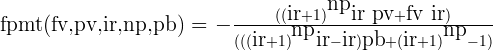 fpmt(1e6,0,.01,120,0)-4347.09484025873
This tells us that to accumulate a million dollars in ten years (120 months) with 12% annual interest in our favor, we need to deposit $4347.09 every month. What if the interest is against us, e.g. -12% per annum — what's the payment then?:
fpmt(1e6,0,-.01,120,0)-14273.0803934121Let's check this result using OpenOffice Calc:
- Entry: =PMT(-0.01;120;0;1000000;0)
- Result: -$14,273.08
Okay, it appears we can create reliable derivative functions using the basic fv equation as our basis. Let's automate the process using a bit of Python. First, a description of the strategy:
- Each function needs a name that differs only a bit from the variable it solves for (it can't have the same name as its result, that would collide with the named argument variables). That way we can remember the function's name without much trouble. Let's name the functions f(name), e.g. ffv, fpv, etc..
- Each function needs an argument list that includes all the arguments except the one it provides.
- So we will use a template string that contains all the variable names, and for each function we'll use regular expressions to create a custom copy of the function string properly formatted for that particular function.
- Then we'll solve the basic fv equation for each desired variable, format the result, and use the solution to define new functions in Sage's global namespace.
- We'll also pretty-print each function as we go.
Here's the code:
fstr = "fq(fv,pv,pmt,ir,np,pb)"
for f in [fv,pv,pmt,np]:
    # make a string version of the target
    fs = str(f)
    # remove from the argument list
    # the variable this function defines
    s = re.sub("%s,?" % str(f),"",fstr)
    # insert the function's name at 'q'
    s = re.sub("q",fs,s)
    # solve for the specified variable
    soln = solve(bffv,f)[0].rhs().exp_simplify()
    # format a function with the solution
    eq = s + " = " + str(soln)
    # create the function in global namespace
    exec preparse(eq) in globals()
    # pretty-print the function
    pps = s + " = " + latex_spc(soln)
    show(pps)
Some very helpful people at the Sage project explained how to create a function from a string describing it (e.g. "exec preparse(eq) in globals()") — I doubt I would have figured that one out on my own. Here's the result:
Needless to say and for the most part, these functions behave very well. One exception is the fnp() function, which requires special handling — for some problems it returns a complex result that doesn't prevent accurate results, as long as the function is wrapped in this way:

Astutue readers will notice I have not defined a function to compute interest rate. As it turns out, this value cannot be acquired with a simple, closed-form equation, instead it must be computed using a root finder. Here is my method to acquire this result:
def fir(fv,pv,pmt,ir,np,pb):
    qf = lambda ir: N(ffv(pv,pmt,ir,np,pb) - fv)
    # never allow ir to equal zero —
    # instead, test ranges on both sides
    try:
        r = find_root(qf,1e-9,100)
    except:
        try:
            r = find_root(qf,-1e-9,-100)
        except:
            print "*** \"ir\" root finder failed. ***"
            r = 0
    return r
Here is a test result:
fir(0, 10000,-100,0,120,0)0.0031141819459532885Let's see how this compares to a spreadsheet's equivalent function:
- Entry: =RATE(120;-100;10000;0;0;0)
- Result: 0.003114181946
There are some special constraints in computing interest rate — the root finder's test values must not be allowed to cross through zero, instead two subranges must be tested separately, positive and negative, each an epsilon away from zero. And there is the possibility of multiple roots, so this particular function isn't particularly reliable, and it isn't deterministic in the way the closed-form functions are.
This page shows an aspect of Sage that makes it far superior to most computer algebra systems — the presence of a well-understood and widely accepted programming language that functions in partnership with Sage's more esoteric features.
Mathematica is a very capable program, but I've never found it easy to write or understand its private, one-off programming language. Python (just below the surface in Sage) is similar to many other computer languages and there is plenty of documentation available to help Sage users learn Python. Solving this financial problem requires a mixture of methods — its solution requires both algebraic and algorithmic manipulations — and this makes Sage an ideal environment for it.
Something missing from Sage that has a bearing on this problem is a way to convert a Sage mathematical function into the syntax common to C, C++ and Java. I'm sure this minor omission will be addressed in a future release, but in the meantime, the plain-text form of a Sage function is so close to the desired syntax that very little effort is required to create it:
bffvfv == ((ir*pb + 1)*pmt - (ir*pb*pmt + ir*pv + pmt)*(ir + 1)^np)/irOkay, that looks promising. Let's try this:
print "double ffv(double pv, double pmt, double ir, double np, double pb) {\n\treturn " + str(bffv.rhs()) + ";\n}"double ffv(double pv, double pmt, double ir, double np, double pb) { return ((ir*pb + 1)*pmt - (ir*pb*pmt + ir*pv + pmt)*(ir + 1)^np)/ir; }That takes us some distance to the goal, but it leaves the Sage exponentiation operator "^" unchanged, which would require some hand-editing to complete the task ( "(ir + 1)^np" -> "pow(ir + 1,np)" ). The point is that 90% of function exportation is nearly automatic, and all of it could be automated with little effort.
"Exploring Mathematics with Sage" by Paul Lutus is licensed under a
Creative Commons Attribution-Noncommercial-Share Alike 3.0 United States License.
| Home | | Mathematics | | * Sage | | | | Share This Page |

