In the previous pages we have shown how to determine a rate of change for our example function, and we have presented a convenient notation for derivatives, as shown below:
(1)
p(t) = t2 (the position function)
(2)
p'(t) = 2 t (the first derivative, velocity)
Higher derivatives are identified as
p''(t),
p'''(t), etc..
Recall that a derivative is a rate of change in a function, and an integral is a history, a summation, of changes that leads to a particular result for a particular argument value, in this example time. To obtain this history, one determines the area under the curve for the function.
Most important of all, and to repeat, an integral and a derivative are
reciprocal operations — if one obtains an integral, then takes the derivative of the result, one gets back what one started with. Once again, this is called the
Fundamental Theorem of Calculus. If, as in our example, one takes the derivative of a position function and obtains a velocity function, one may integrate the velocity function to reacquire the position function.
This page discusses a widely used numerical method for integration, a method used in cases where a function does not have another function as its integral. As it turns out, and just as with derivatives, there are ways to obtain a function, rather than a number, that represents the integral for many functions, and this outcome is of course preferred. But there are many other functions that have no symbolic integrals, and such functions must be evaluated numerically, using methods like that presented on this page.
Fortunately there is a geometric relationship between a function and its integral that is easy to express, if not always easy to compute — as explained above the integral of a given function is equal to the area under the curve of that function. This relationship is shown in the graphs on this page. The numerical method obtains an estimate of the area under the curve by creating a series of rectangles and summing their areas.
Graph 4: Estimating the area under a curve
|
|
Time
|
Height
|
Width
|
Area
|
|
2.0
|
4.0
|
4.0
|
16.0
|
|
6.0
|
36.0
|
4.0
|
144.0
|
|
10.0
|
100.0
|
4.0
|
400.0
|
|
Total
|
|
|
560.0
|
|
Error
|
|
|
-2.86%
|
Graph 4 data table
|
Graph 5: Using smaller steps
|
|
Time
|
Height
|
Width
|
Area
|
|
0.5
|
0.3
|
1.0
|
0.3
|
|
1.5
|
2.3
|
1.0
|
2.3
|
|
2.5
|
6.3
|
1.0
|
6.3
|
|
3.5
|
12.3
|
1.0
|
12.3
|
|
4.5
|
20.3
|
1.0
|
20.3
|
|
5.5
|
30.3
|
1.0
|
30.3
|
|
6.5
|
42.3
|
1.0
|
42.3
|
|
7.5
|
56.3
|
1.0
|
56.3
|
|
8.5
|
72.3
|
1.0
|
72.3
|
|
9.5
|
90.3
|
1.0
|
90.3
|
|
10.5
|
110.3
|
1.0
|
110.3
|
|
11.5
|
132.3
|
1.0
|
132.3
|
|
Total
|
|
|
575.0
|
|
Error
|
|
|
-0.17%
|
Graph 5 data table
|
|
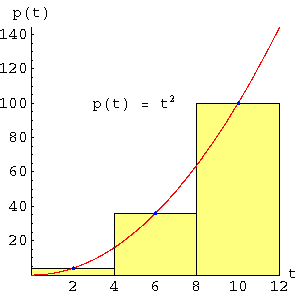
Examine Graph 4. This represents our first, coarse effort to obtain the area under the curve of our function. As one can see, the method relies on rectangles that occupy most of the area under the function's curve.
While examining Graph 4, pay attention to the rectangle at the right, the one lying between t = 8 and t = 12. Notice that a large part of this rectangle is above the function's curve (at the left), while much of the right side is below the curve. This may seem to undermine the goal of accurately estimating the area under the curve, until one realizes that the area outside the function's curve at the left may be thought of as a triangle, one that can be rotated clockwise through 180 degrees, pivoting around the blue dot at t = 10, and placed on top of the rectangle at the right. This same argument applies to the other rectangles, making them seem more appropriate as stepwise approximations of the curve's area than it may appear at first glance.
To begin our numerical analysis, it should be pointed out that the integral of
t2 with respect to
t is known, it is equal to
t3/3. The exact area under the example graphs on this page is therefore equal to:
| (3) | t3 | = | 123 | | = 576 |
 |
|
| 3 | 3 | |
This means we have an accurate result for comparison purposes. It is important to add that not all functions can be integrated symbolically (e. g. in a way that produces a function as a result), so it is frequently necessary to use numerical methods such as we are discussing. In Graph 4 we see three rectangles that have the areas listed in the Graph 4 data table. When we add the areas together, we see that the result differs from the true area under the curve by -2.86%. This error is caused by the relatively small number of rectangles used in Graph 4.
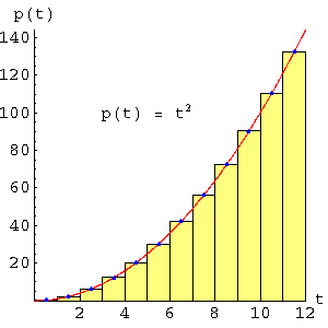
In the second example, shown in Graph 5, we use more rectangles in an effort to more closely match the function's curve. In the Graph 5 data table we see the error has diminished to -0.17%
At this point it should be clear that, just as with derivation, if we take smaller steps, we get more accurate results. And, just as we saw when computing derivatives, we can use the concept of a limit to make a statement about an arbitrarily large number of rectangles in order to approach the exact area under our curve:
|
(4)
|
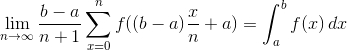
|
Two new symbols are introduced in this equation. The first, Σ, is the Greek letter Sigma. It is used to express a summation of terms between specified endpoints (shown above as
a and
b). It is used here to describe the method of summing rectangles. The second symbol, an elongated "s" at the right, is the symbol for integration. If we were to express this entire equation in words, we might say, "As the number (
n) of rectangles approaches infinity, the outcome approaches the integral of a function f on the interval between
a and
b".
At this point, the reader should have acquired a general sense of what a derivative and an integral are, and may have acquired an instinctive sense of their relationship. We will now turn to some applications of these methods and consider what tools are available for handling Calculus problems.


 Share This Page