

 Share This Page
| Home | | Mathematics | | | | Share This Page |
Copyright © 2014, Paul Lutus — Message Page
(double-click any word to see its definition)
Click here to download this article in PDF form
NOTE: This article covers methods applied to continuous statistical distributions. For discrete-value statistical analysis, my Binomial Probability article is probably a better choice.
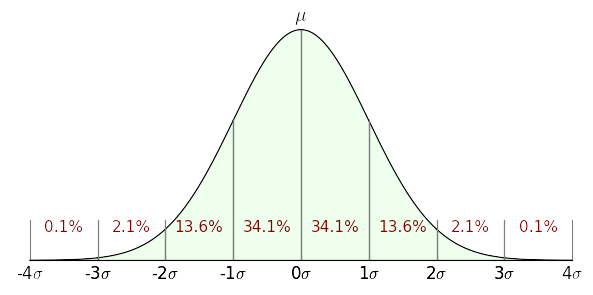
Figure 1: Graph of a normal or Gaussian distribution (σ = unit of standard deviation)
This article introduces, and provides online tools for the exploitation of, the normal or Gaussian distribution ("bell curve"), a key idea with wide application in modern statistical analysis. Topics covered include a summary of the underlying theory, online calculators for analyzing statistical results and reducing data sets to their statistical properties (mean, variance, standard deviation, standard error), an in-depth mathematical description of the methods underlying the Guassian distribution, and a discussion of algorithm design.
The goal of statistical analysis is to be able to make general statements about a modeled system based on limited samples. A surprising number of natural systems and processes can be successfully characterized by analysis of a limited set of measurements using a Gaussian-distribution model (Figures 1 and 2).
For an example of how often one encounters a Gaussian distribution in nature, Figure 2 models a "random walk" consisting of, in a manner of speaking, many flips of a fair coin that guide the steps of a random walker initially located at the central location marked "μ". If the random coin flip comes up "heads", the walker takes one step to the right, otherwise left. At the end of the walk, the column nearest the walker's final position becomes taller. Even though the process is entirely random, the outcome approximates a Gaussian curve.
The elements in this class of statistical analysis are:
- An average or "mean" value, the sum of the values divided by their number.
- A "variance", which quantifies how much the samples differ from the mean value.
- A standard deviation, which is the variance in a more useful form.
- A standard error, an indication of how well the analysis reflects reality.
With these values in hand, one can predict the properties of the system from which the measurements were acquired. Here's an example — let's say you build widgets that are expected to be 100 cm long but that, when constructed, have some variation in their lengths. You want to be able to predict the number of production rejects based on quality control acceptance limits and a limited set of production measurements. Using statistical analysis methods, you would:
- Acquire a set of measurements of typical manufactured items, as many measurements as practical.
- Process the data set and acquire mean, variance and standard deviation (square root of variance) values using a data processor like that included in this article.
- Use the acquired values, the established manufacturing aceptance limits, and a Gaussian curve calculator (also included in this article) to estimate the rate of manufacturing rejects.
The above is just an example of statistical data analysis. There are many applications for these methods in everyday life — measures of people's height, weight, IQ, and many similar quantities are appropriate to these methods and can provide insight into them.
It should be noted that this kind of statistical analysis has a degree of uncertainty related to the number of samples or measurements taken. In the analysis method described here, this uncertainty is quantified by the "standard error" value, which is computed along with the values described above and which provides a measure of confidence in the analysis.
Analysis based on a normal or Gaussian distribution is most appropriate for data sets having an innate normal distribution of its own, that is to say, a centrally weighted grouping of data with decreasing examples far from the average value of the data (the "mean"). Figure 1 shows the proportions and percentages one expects to see in a data set for which a Gaussian analysis is appropriate.
Caveat: it cannot be overemphasized that many data sets have properties that make them unsuitable for this treatment, and there are any number of stories of misapplication of the Gaussian distribution where another kind of analysis would better fit the data and circumstances.
A normal (Gaussian) distribution is defined this way:
(1) $ \displaystyle f(x,\mu,\sigma) = \frac{1}{\sigma \sqrt{2 \pi}} e^{-\frac{(x-\mu)^2}{2 \sigma^2}} $Where:
- $e$ = base of natural logarithms.
- $x$ = argument.
- $\mu$ = (Greek letter mu) mean or average value.
- $\sigma$ = (Greek letter sigma) standard deviation (σ2 = variance).
If $\mu$ = 0 and $\sigma$ = 1 the distribution is called a standard normal distribution or unit normal distribution. This special form is to statistics what a normalized function is to general analysis — a function whose range of values is normalized to the multiplicative identity (i.e. 1) to maximize flexibility. The unit normal distribution has this abbreviated definition:
(2) $ \displaystyle f(x) = \frac{1}{\sqrt{2 \pi}} e^{-\frac{x^2}{2}} $Computing an Area
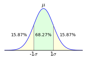 Figure 3: Area bounded by ±1σ
As it happens, computing a single value on the normal distribution is easily accomplished using one of the above equations, but many statistical problems require that one compute an area with a definite integral. For example, given an analysis of population IQ scores that produces a mean (μ) of 100 and a standard deviation (σ) of 15, one might want to know what percentage of the population is predicted to lie between scores of 85 and 115. To solve such a problem, one would use this form:
(3) $ \displaystyle f(a,b,\mu,\sigma) = \int_a^b \frac{1}{\sigma \sqrt{2 \pi}} e^{-\frac{(x-\mu)^2}{2 \sigma^2}} dx $To apply equation (3) to the above-stated IQ problem, one would provide these arguments:
- a = 85 (integral lower bound)
- b = 115 (integral upper bound)
- $\mu$ = 100 (mean)
- $\sigma$ = 15 (standard deviation)
The result for these arguments is approximately 0.6827, a canonical numerical result with which my readers will likely become familiar over time — it's the area of the unit normal distribution between -1σ and 1σ (Figure 3). Expressed another way, this is the two-tailed outcome for a standard deviation of 1, or the proportion of population values that lie within ±1σ (standard deviation) of the mean.
68-95-99.7 Rule
This might be a good time to briefly address the so-called 68-95-99.7 rule. In statistical work, it is common to ask what proportion of the measured population's values lies within particular bounds. Refer to Figure 1 above to see the relationship between σ (standard deviation) values and corresponding areas of the normal distribution. For example, it seems that 34.1% of the values lie between 0σ and 1σ — this is called a one-tailed result. For the more commmon two-tailed case shown in Figure 3, in which the area between -σ and +σ is taken, here are some of the classic values:
Note about Table 1 that the value column refers to the total area outside the specified ±σ bounds. For example, in the earlier IQ problem, we found that 68.27% of the population have IQs between 85 and 115. This means 31.73% of the population have IQs that are either above or below this range (15.87% below, 15.87% above). (I hasten to add that the IQ problem is hypothetical — IQ scores cannot be reliably fit to a normal distribution in such a simple way.)
±σ value value 1 68.27% 31.73% 2 95.45% 4.55% 3 99.73% 0.27% 4 99.99% 0.01% Table 1: Normal distribution areas for ±σ argumentsAlgorithmic Limitations
Let's turn now to the problem of creating practical numerical results. Unfortunately, in a much-lamented limitation of Calculus, no closed-form integral exists for equation (3) shown above — one must use a numerical method to acquire an approximate result. Because of the importance of this integral to applied statistics, a carefully designed numerical function is provided in many computing environments named the error function, erf(x), with this definition:
(4) $ \displaystyle \text{erf}(x) = \frac{2}{\sqrt{\pi}} \int_0^x e^{-t^2} dt $Remember again about erf(x), notwithstanding that it can be expressed so easily, that it has no closed-form solution and one must use numerical methods to acquire approximate results. Using erf(x), one would express equation (3) this way:
(5) $ \displaystyle f(a,b,\mu,\sigma) = \frac{1}{2} \, \text{erf}\left(-\frac{\sqrt{2} (a - \mu) }{2 \,\sigma}\right) - \frac{1}{2} \, \text{erf}\left(-\frac{\sqrt{2} (b - \mu)}{2 \, \sigma}\right) $For the IQ problem described above, in a computing environment one would acquire a result this way:
(6) y = f(85,125,100,15) (with result 0.6826895)To convert the outcome of equation (6) into a practical result, one need only multiply it by the population size. For example one might ask, of a population of a million people, how many have an IQ at or above 135? Assuming that our statistical parameters are legitimate, we can calculate:
(7) y = f(135, 1000000 ,100,15) * 1000000 (with result 9815.32)Notice about this result that an arbitrary constant was used for the upper bound. Ideally, one wants to compute the area between 135 and +infinity, but in a computing environment, one must choose a finite value to approximate infinity.
This section has a Gaussian curve calculator able to produce results for the equations and methods described above. With appropriate data entries the calculator can answer practical questions like these:
Problem a b μ σ p For the unit normal distribution, what percentage of the samples lies between -1σ and +1σ? -1 1 0 1 100 In a population of one million people, given an IQ μ of 100 and σ of 15, how many people have an IQ at or above 135? 135 1000000 100 15 1000000 In a manufacturing process, a widget's variable dimensions fall on a normal distribution. Production measurements show that the part's average length is 100 cm and the standard deviation is 2 cm. The manufacturing acceptance bound from the mean is ±2.5 cm. What percentage of the parts are likely to be accepted? (Note that in this problem, $\overline{r}$ = percentage rejected.) 97.5 102.5 100 2 100 To justify announcing a new discovery like the Higgs Boson, experimental physicists require that their data have a p-value equal to or less than 5σ. What is the numerical value of 5σ when expressed as a p-value? (Click here for a more detailed description of this problem.) 5 1000000 0 1 1 Feel free to compute solutions for problems of your own. Enter values into the green data windows, then press Enter or press the Compute button:
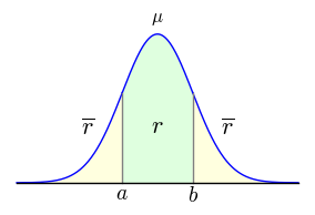 Figure 4: Graph showing relationship
between $a$, $b$, $r$ and $\overline{r}$
The above calculator and exposition show how to analyze and interpret the values (mean and standard deviation) derived from data acquisition and processing. This section shows how to acquire and process the required data. (The order of this article's topics is intentional — it's easier to understand how to apply mean and standard deviation values than it is to process the data required to obtain them.)
Equations
While processing a data set, one acquires and then exploits the following quantities:
Name Method Comment n n = Number of samples Sample size, used in all later steps. $\mu$ $ \displaystyle \mu = \frac{\sum{x}}{n}$ Mean (average) value: the sum of data values divided by sample size n. $v$ $ \displaystyle v = \frac{\sum{(x-\mu)^2}}{n}$ Variance: Sum of differences squared divided by sample size n. $\sigma$ $ \displaystyle \sigma = \sqrt{\frac{\sum{(x-\mu)^2}}{n}}$ Standard deviation: square root of sum of differences squared divided by sample size n. $v_u$ $ \displaystyle v_u = \frac{\sum{(x-\mu)^2}}{n-1}$ Unbiased1 variance: Sum of differences squared divided by sample size n-1. $\sigma_u$ $ \displaystyle \sigma_u = \sqrt{\frac{\sum{(x-\mu)^2}}{n-1}}$ Unbiased1 standard deviation: square root of sum of differences squared divided by sample size n-1. se $ \displaystyle se = \frac{\sigma}{\sqrt{n}}$ Standard error: standard deviation divided by square root of sample size n. 1 The terms "unbiased sample variance" and "unbiased standard deviation" are more fully explained here. User Data Processor
The above methods and equations are computed by the data processor below. Just enter (or paste: Ctrl+V) data into the green data window, then press "Compute" to acquire a result:
Discussion
The data processor above has a control to adjust the sample bias in the range {-1,1}. After much reading on this topic, and after seeing a number of different terms for the same things used by different authors, I decided I wasn't going to be able to provide a predefined set of options that would satify everyone. Just remember that the bias control influences the variance and standard deviation in various ways confusingly explained here.
The data processor's results can be exported intwo ways:
- The user can click the "Transfer" button to transfer mean (μ) and standard deviation (σ) results to the Gaussian curve calculator that appears earlier in the article.
- The user can pass his mouse cursor across the results window, then press Ctrl+C to copy the result table to the system clipboard.
Remember that large data sets produce smaller standard error values, reflecting the idea that more samples should increase the accuracy of the result. But there's another use for standard error and different sized data sets — one can submit a small data sample to the processor, record the mean and standard deviation values, then increase the size of the data set to see if the mean and standard deviation change significantly. This procedure is meant to discover how many measurements are required to produce reliable results.
The algorithms that power this page are located here, a JavaScript source file released under the GPL. The source has these main sections:
- Stats.calc() provides the Gaussian curve calculation functions.
- Stats.process() provides the data processor functions.
- Stats.animate() provides the graphics functions used by Figure 2 above.
The calculator requires an embodiment of the error function, provided here by Stats.erf() and Stats.erfc(). Again, integrating the Gaussian curve must be performed numerically, which leads to a certain amount of algorithmic complexity.
I have created other versions of the gaussian curve calculator:
- This Python script relies on the extensive Python scientific and technical libraries to provide the Gaussian calculator functions with much less complexity.
- This Python script produces the same results as the above data processor.
- This Java calculator project includes a statistics section that provides the same functions, but with the same level of complexity as the JavaScript source for lack of adequate high-level libraries in Java. Unfortunately because of security issues, Java applets are no longer a practical way to deliver technical Web content, but the calculator still works as a desktop application.
The statistical data processing is comparatively straightforward and should be easily understood by reading the JavaScript source.
| Home | | Mathematics | | | | Share This Page |